HMPI kirsten, Author at HMPI

H.E. Frech, III, University of California, Santa Barbara; Mark Pauly, The Wharton School, University of Pennsylvania; William S. Comanor, UCLA Fielding School of Public Health; and Joseph R. Martinez, Jr. The Wharton School and Perelman School of Medicine, University of Pennsylvania

Contact:pauly@wharton.upenn.edu

Abstract

What is the message? Pharmaceutical prices are set through interactions among drug companies, the sellers, and health insurers. This study offers a series of models demonstrating the impact of monopoly prices on insurance coverage and the consumer.

What is the evidence? An analysis of patented drugs with no close substitutes sold by monopoly drug firms to competitive private insurance plans and the effects of insurance-induced price effects on subsequent changes in co-insurance rates.

Timeline: Submitted: June 10, 2023; accepted after review Sept. 1, 2023.

Cite as: H.E. Frech, Mark Pauly, William S. Comanor, Joseph Martinez. 2023. Consumer Welfare, and Market Equilibrium in Private Insurance Coverage of Patented Drugs. Health Management, Policy and Innovation (www.HMPI.org), Volume 8, Issue 2.

Download PDF

Background and Insured Patient Demand

Private sector insurers are under intense pressure to restrain premium growth in both individual and group markets, especially with regard to pharmaceutical spending. Such growth is largely driven by the diffusion of costly new products, especially by novel brand-name, patent-protected prescription drugs, and by increases in the prices of products or services where there is little competition. Historically, U.S. insurers, public and private, have taken a passive role with regard to the prices or quantities of effective branded drugs with no close clinical substitutes. (They might use formularies tiered with copays and reference prices for products for which there were alternative clinical choices (Cremer and Lozachmeur), but that is not the case to be considered here.) Once approved by the FDA, insurers would generally pay for whatever drugs physicians and patients agreed to order at whatever price the drug firm charged. Historically, drug insurance policies often included uniform coinsurance or other forms of cost sharing that applied to all prescription drugs, so consumers were partially exposed to high prices and deterred from higher quantities of covered drugs. This exposure is heightened in modern health insurance, where most policies include drug coinsurance, and few drugs are excluded from coverage.

In this paper, we present a set of models of simultaneous determination and market equilibrium for drug firm price and insurance coverage for “exclusive” branded drugs, those with no close clinical substitutes (new molecular entities or biological products). Such breakthrough drugs constitute a substantial share of the growth in drug spending. Insurers also find their prices difficult to modify even when the insurer has a large market share (Lakdawalla and Yin, 2015). We will explore simple monopoly pricing by the drug firm that insurers are assumed to take as given, but with insurer choice of cost sharing (given the price set by the monopolist) as a way of increasing the welfare of risk-averse consumers. The drug firm is assumed to set the simple monopoly price given demand and a constant (zero) marginal cost of production and distribution.[1] After developing this benchmark model, we will comment on the impact of moving to alternative pricing models for drugs when insurers take a less passive approach with regard to drug price and quantity.

To focus attention on payment mechanisms, we present a benchmark model in which we assume that drug insurance markets are approximately competitive, with no single insurer having a large enough market share among insurance buyers in that location to motivate face-to-face bargaining with any drug firm. Some insurers are national firms (that own pharmacy benefit managers) but they typically tailor their plans to the demands of local employment-based groups. This assumption allows us to avoid the often-intractable problem of modeling bargaining equilibria in a drug monopoly-insurance monopsony setting.

Our approach will differ from most other commentary on drug pricing and its relationship to insurance (Berndt, McGuire, and Newhouse, 2011; Danzon and Pauly, 2002) by going beyond discussion of what insurance buyers might do when a new drug is introduced at some (high) price. We ask how the seller’s price responds to the insurance they choose. We then take the next step and ask how the coverage chosen may change in response to the new price and trace out the independent adjustment process to an equilibrium in seller price and insurance coverage. To our knowledge, modelling the steps of subsequent insurance firm and buyer responses to the insurance-induced increase in branded drug prices along a linear demand curve is a novel contribution, as is the specification of an equilibrium in which the market price and the market level of insurance are mutually consistent.

More specifically, we will deal with the challenging case in which drug firms set prices of branded products based in part on insurance coverage design, while insurers seek to offer cost-sharing designs that patient-consumers will prefer, given the consumers’ financial risk associate with a given drug firm price and illness-affected quantity demanded at that price. We focus on a major paradox in the simple monopoly model which has not been recognized: when coverage and price are endogenous, market equilibrium outcomes may leave representative risk-averse consumers worse off or no better off with than without insurance. Alternatively, market equilibrium may not exist.

Modelling

Initial Assumptions

Our focus is on a hypothetical market of competitive profit-maximizing private insurers who can offer varying cost-sharing levels for different drugs and who can refuse to cover a product at all (100% cost sharing), Following a long line of literature, we simplify insurance by treating all cost sharing as a coinsurance percent or proportion (Zeckhauser, 1970; Feldstein, 1973; Feldman and Dowd, 1991).[2] The insurance product is demanded to treat an uncertain illness of potentially varying severity, and risk-averse consumers may demand insurance to cover the financial cost of the drug when they use it. We assume a linear demand curve both because it is a simple way of illustrating consumers’ surplus diagrammatically and because the property of high elasticity and high prices and low elasticity at low prices seems most realistic when quantity demanded is bounded by zero and use by all persons with an illness. Insurance demanders, who might be individuals or homogenous groups of individuals, can then choose which combination of coverage and associated premium they most prefer, prior to knowing whether they will get the illness and how severe it will be.

The drug to be covered is sold by a profit-maximizing firm, which has market power because it has a patent on an exclusive drug. In order to characterize a demand curve facing these firms, it must be the case that different potential buyers attach different values to a given product once illness has occurred because it yields different amounts of increased expected health [quality-adjusted life years (QALYs] depending on illness severity. If all persons with the illness a drug treats expect to gain the same number of QALYs from treatment, and have the same monetary value per QALY added, the seller would face a horizontal demand curve and either sell none of the product or sell it to all those with the illness, depending on where it set the price (Pauly, Comanor, Frech, and Martinez, 2021). In what follows, we assume instead that severity (and marginal benefit) varies after illness strikes but that monetary values of QALYs are the same across buyers of drugs and insurance.

We also assume for simplicity that each individual insured person consumes either zero or one drug treatment (Garber, Jones, and Romer, 2006). This allows us to focus on the extensive margin in describing the demand curve for the product. We use a standard two-state expected utility maximization model with moral hazard. For ease of exposition, we ignore income effects on demand and, in most cases, set marginal cost to zero.

The model

Following Feldman and Dowd (1991), we define the “risk premium” π as the value subtracted from income in the no-illness state that equates an individual consumer’s expected utility with insurance and some coinsurance rate of c to the expected utility without insurance, or:

(1) E[V( X- π- (1 – c) E (PM) – cPM + W(M)] =E [V(X-Pm) + W(m)]

Where the utility function is assumed to be separable into two parts, V and W, X= income, c = coinsurance rate, P =gross price of treatment, M= quantity with this insurance, and m = quantity without insurance. Equation (1) also assumes that the insurance is actuarially fair so that the premium K=E[(1-c)PM].

Then it can be shown (Cf, Feldman and Dowd, 1991) by a second order Taylor series expansion of (1) that π is given by:

(2) π = [[E(P(m-M)]+ [E(W(m)]-EW(M)]/V’] + (Rσ²)/2.

Here the first term in brackets represents the difference in expected spending, the second term represents the difference in value of care received (difference in utility divided by the marginal utility of income), and the last term represents the value of risk reduction from insurance, where R equals the Arrow Pratt coefficient of risk aversion and σ² is the variance of out of pocket spending.

The insurance buyer maximizes expected utility by choosing the level of c which maximizes π, the net gain from insurance. Risk arises in this setting because illness is uncertain, its severity conditional on its occurrence is uncertain, and therefore the out-of-pocket spending by the insured is uncertain. Moral hazard arises when the insurance payment is made conditional on the level of care chosen post-purchase and when the severity of illness (or other determinant of care demand) is then only known by the insured but not by the insurer. One of our primary interests in this paper is in the change in medical care use that is incentivized by insurance and resulting consumer welfare cost, so our discussion will be primarily about the first two terms of expression.

To explore the impacts of variation in coinsurance and resulting changes in monopoly price on the risk premium for the representative consumer, we follow Feldman and Dowd in relying on an analysis of the geometric welfare triangle that shows how consumers’ surplus changes when market-level coverage and price change. We then compare that change with changes in the value of risk reduction from insurance. We differ in that we assume that the drug firm charges the same price to the insured and the uninsured.

Equilibrium and consumers’ surplus without insurance

If there were no insurance (or if insurance could take the form of fixed dollar indemnities conditional on the patient’s state of health and the type of illness), the resulting demand curve for the product, which is also the schedule of marginal health benefits, would (ignoring income effects) be the one which would prevail in a simple monopoly market. The drug firm would then set its profit-maximizing price, and patients would choose whether or not to demand the drug at that price. Note that, at the profit-maximizing price, the demand curve will be elastic: if the price is raised above this price enough, consumers will not buy the drug to such an extent that drug firm revenue will fall. (The drug monopolist can set any price it wants but it cannot sell any quantity it wants.) As usual, at the monopoly price there is welfare loss because of this demand response. Consumers’ surplus would be lower than if the price were competitive.

This scenario of simple monopoly without insurance predicts a price in excess of marginal cost, but one at which those consumers who do choose to buy the product obtain positive consumer surplus, on average, compared to a situation in which the drug was not available. Many pay less than the value of the benefit they expect to get from the drug. In what follows, we assume that the marginal cost of the drug is zero so that profit and revenue maximization coincide. Consumers’ surplus would be maximized if 100% of patients with the illness obtained the drug, but that will not happen in a simple monopoly equilibrium.

Adding insurance with independent adjustment by the drug seller and the buyers of insurance

Because insurer information on the state of a person’s health is imperfect, health insurance cannot take the form of predetermined indemnity payments conditional on the health state. Instead, as noted above, we model insurance coverage as using proportional coinsurance to limit moral hazard, with the choice of treatment quantity, given insurance coverage, to be chosen by a patient-doctor agreement influenced by the level of the out-of-pocket payment. (If the patient knew the health state prior to purchasing insurance but the insurer did not, the situation would be one of adverse selection.) The patient and physician are assumed to observe the health state (illness severity) with full accuracy once an illness has occurred. Given the assumption that each person demands one or zero units of drug treatment, the firm and market demand curve for the product without insurance will track the distribution of health benefits from the drug in a given population. If we assume that these benefits are determined by illness severity—sicker people get more benefit from the drug—the market demand curve is defined by the distribution of illness severities. There will be some price so high that no consumers, not even the sickest, will choose to buy the drug, and at a near zero price all members of the population with the illness will buy the drug but no one who is not sick will choose it. The demand curve strikes both price and quantity axes.

We model the choice by risk-averse consumers facing a tradeoff between lower coinsurance (and therefore lower variance of out-of-pocket spending) against greater moral-hazard-caused reduction in consumer surplus. To determine the market equilibrium for insurance coverage and price of this drug, we assume there are numerous insurance purchasers and competing insurers who take the drug seller’s current market price as given, and have no foresight about future drug firm price changes. This is the standard Nash assumption.

Begin by assuming that the drug firm faces a known linear demand curve for drugs and that the no-insurance simple monopoly price prevails. Insurers offer coverage with the coinsurance rate that is optimal at that price for consumers, given the consumers’ expected marginal benefit curve from the product and given their degree of risk aversion. That would be the level of coinsurance that would maximize the risk premium, given the initial price (the no-insurance price). Thus, the coinsurance rate is determined by consumer preferences. The monopoly seller now faces a different demand curve with P replaced by P/c. This is the equilibrium described by Garber, Jones and Romer (2006).

Figure 1 illustrates the standard argument about the effect of coinsurance on market equilibrium quantity and price. P* is the no-insurance monopoly price. At this price, 50% of patients with the illness buy the drug. The triangle A represents the welfare loss from monopoly pricing. Now suppose that risk-averse consumers choose insurance with the coinsurance c* that maximizes expected utility in equation (2). The presence of insurance will then cause the demand curve faced by the monopolist to rotate upward as indicated. A profit-maximizing seller will react to the demand curve affected by coinsurance by increasing the price to a new higher profit-maximizing level. In figure 1, this change is shown by the pivoting of the demand curve around the x-axis intercept (Pauly, 2012) leading to a new monopoly price, P’. At this new monopoly price P’ and the original coinsurance rate c*, the net price settles to the same level as the gross price before insurance. The quantity with insurance is then the same quantity (50% of patients using the drug) as without insurance.

However, this is not the end of the story. What happens next to the coinsurance rate chosen by the representative risk-averse consumer after the increase in price is ambiguous in theory (Phelps, 1973). The desired level of the coinsurance rate may either rise or fall with increases in the market price. Roughly speaking, the direction of this change depends on the representative person’s marginal value of risk protection relative to the cost of moral hazard; coinsurance will increase if the former is smaller relative to the latter—and vice versa.

Let us first consider the case where the coinsurance rate increases if P increases. Demanders of insurance may choose this level of coverage because there is a larger marginal welfare loss at a higher price, and that larger welfare loss may more than offset a higher level of financial risk. If coinsurance rises in the market, the drug firm would reduce its price. However, after this increase the user price will again end up at the original gross price. Then coinsurance rises a little again, and the process continues by smaller and smaller steps until it converges to a Nash equilibrium of drug prices and coinsurance. In that independent adjustment equilibrium (if it exists) the level of coinsurance will be optimal for consumers given the drug price, and the drug price will be profit-maximizing for the drug firm given the coinsurance affected demand curve. Formally, the representative consumer chooses the utility maximizing level of coinsurance, given P, described in equation 2 while the drug firm chooses the level of price, given c, which satisfies the usual MR =MC condition with gross price defined as P/c. More importantly, the net price to consumers in the final equilibrium (as in all other stages) is at the same level as the gross user price before insurance was available, and the equilibrium quantity of the drug purchased by 50% of those at risk.

Figure 2 illustrates. It shows the independent-adjustment (Cournot-Nash) process. Following the textbook model (Emerson, 2018), there are two best response reaction curves: one for the drug firm (profit maximizing price given coinsurance) and the other for the representative insurance buyer (expected utility maximizing coinsurance rate given price). The path of prices and coverage given some initial starting point value for c is shown, and the process converges to equilibrium at the intersection point E in this example.

The paradox

We now note a major issue: in this equilibrium (if it exists), the user price equals the initial no-insurance price, and so the quantity demanded is the no-insurance quantity (50% of the population covered). This leads to:

Proposition 1: Compared to the no-insurance equilibrium, in the insured Nash equilibrium (if it exists), consumers end up with the same expected quantity of care, (at which 50% of patients with the illness use the drug), and the same expected distribution of out-of-pocket payments.

This positive proposition may appear fairly obvious, though to our knowledge it has not been noted in the literature. What is less obvious and more paradoxical is the welfare implication:

Welfare Implication 1: In equilibrium consumers are worse off with some insurance than with no insurance. They experience the same out-of-pocket cost, financial risk, and the same quantity as with no insurance, but pay more in premiums.

Why does insurance fail to provide additional risk protection compared to the risk averse consumer’s situation without insurance? The reason is because insurance continues to change the demand curve in ways that raise the monopoly price unless and until the consumer cuts back far enough on insurance coverage. Increasing coinsurance has to catch up with rising prices. In this equilibrium with insurance, the seller now collects in out-of-pocket payments and insurance benefits a total amount which is (potentially much) more than the no-insurance revenue. This inferior equilibrium is still stable because, at the higher product price, consumers will want the insurance they have. However, if the government would forbid the sale of insurance, all consumers would be better off.

Nature and existence of equilibrium

Now suppose that the initial level of ideal coinsurance (given P) was less than 0.5. This implies that after coverage is purchased the profit-maximizing price will be greater than 2P. At that price, the quantity will be 50%. However, at that price and quantity, the consumer will be worse off from purchasing the insured drug. There will not be an equilibrium. In the next round the drug seller will reduce the price to P, the consumer will again choose c less than 0.5, and the process will repeat.

Hence:

Proposition 2: Equilibrium does not exist if the consumer chooses coinsurance at or below 0.5 or if the consumer reduces desired coinsurance as price increases.

If the consumer responded to the higher monopoly price by choosing a lower coinsurance rate, that choice will lead to even higher prices and premiums which will lead to zero insurance. At zero insurance price will fall back to the simple monopoly price, and then buyers will demand insurance with coinsurance below 0.5. Hence the price will move from the simple monopoly price to a price that exceeds the reservation price, and back again—independent-adjustment equilibrium without foresight will not exist.

Adding foresight

It is plausible that the drug monopolist will anticipate future changes in market levels of coinsurance when it changes its price (even if an individual competitive insurer might not anticipate further changes in the drug firm’s price in response only to its own coverage change). That is, the drug seller may know what levels of coverage for its drug (including no coverage) insurance buyers will choose at a given launch price or subsequent price. In the case where coinsurance is increasing in P, a drug seller strategy alternative to the independent adjustment process just described may simply be to set the price at what would be the equilibrium of that independent adjustment process. At that price insurance demanders will choose the coinsurance level that is optimal, and the quantity level of 50%. The outcome will be the same as that previously described but will converge immediately.

The more challenging case is when desired coinsurance falls as price increases. The outcome of no insurance and no drug use is clearly inferior to some other option with a particular price P* and some other level of coinsurance. But if that combination is put in place, buyers of competitive insurance will want more generous coverage and insurance firms will see positive prospective profits from offering it. Prices and coverage will continue to rise to such an extent that no insurance (and no drug purchase at a very high price) is preferable to keeping insurance. When consumers drop all coverage price will fall but that is also not an equilibrium, so the cycle begins again.

As before, foresight may come to the rescue here. The drug firm may choose a price at which buyer insurance coverage and quantity demanded at that price still yields consumers surplus.

From passive to active

Might an individual competitive insurer in at the equilibrium coinsurance rate gain by proposing to the drug seller an alternative arrangement with a new insurance product that carries a lower coinsurance rate in return for the drug seller’s promise to charge a lower price? It is commonly believed that an insurer needs to enroll a large share of the users of a branded drug to negotiate with the drug firm — “to be effect as negotiators in pharmaceutical markets, PBMs need size” (Werble, 2017). Is this necessarily true? Might this kind of price negotiation prevail even if each insurer has only a small market share and hence no bargaining power?

The answer turns out to be affirmative. We begin in a Nash equilibrium with a given coinsurance rate c₀ and a given gross price P₀ with quantity Q₀=0.5, at which marginal benefit and user price is c₀P₀. This yields drug firm profits of P₀(0.5). Now consider an offer from the insurer to pay a lower gross price P₁ but demand a higher quantity Q₁ such that drug firm profits are marginally greater than in the Nash equilibrium. That is, the increase in quantity from 0.5 to the larger quantity patients will demand with a lower gross price and lower coinsurance (DQ) exceeds by a small amount e the fall in profits on the original quantity from the reduction in gross price DP.

(3) DQ(P₁) – DP(0.5) = e.

The insurer agrees to adjust coinsurance so that demand at gross price P₁ does indeed equal Q₁ at that price. Call this new user price c₁P₁ (This level of coinsurance would generally be lower than the level on the reaction curve at P₁ so it is not a Nash combination.) Hence the user price falls from c₀P₀ to c₁P₁.

At this new point the seller has somewhat higher profits. What is the change in total surplus DCS? It is the change in payments to the insurer, or e above, plus the increase in expected consumers surplus which is:

(4) DCS = 0.5[c₀P₀(0.5)]-[(0.5-DQ) c₁P₁]

The first term in square brackets is the increase in expected consumers surplus if the user price were reduced from the original level c₀P₀ to zero and quantity increased from 0.5 to 1, and the second term is the shortfall from that amount because user price remains positive at c₁P₁.

That is, the representative insureds consume a larger quantity of care whose value is positive even after paying off the monopolist; they expect more consumers surplus. Hence both sellers of the drug and buyers of insurance are better off at this point than they were in Nash equilibrium. Of course the best deal for insured consumers would be one in which user price was zero (equal to MC) and Q=1 (100% of those who got sick and could benefit from the drug).

We can think of the drug firm’s response to the insurer’s offer as movement along an all- or-nothing supply curve (Friedman, 1976; Herndon, 2002) along which the required quantity is so large that, at the proposed (lower) per unit price, the seller is just indifferent between accepting the offer and staying at the previous equilibrium (or the chaos of the non-equilibrium case). Effectively, this alternative is identical to proposing a lump sum amount (unit price times maximum quantity) that extracts almost all supplier surplus from the seller. This is also a step in the direction of the two part model of Lakdawalla and Sood (2013).

If one thinks of the drug company as suggesting this type of deal as an improvement from the Nash equilibrium (or non-equilibrium), the drug company would get more surplus and the insurer and its members would be indifferent or near indifferent. It is also possible that insurer and the drug company share the surplus gained by this sort of deal.

Empirical evidence

There is evidence consistent with some of the steps in the adjustment process to independent adjustment equilibrium. There is time series evidence that more generous market-level insurance coverage is associated with higher prices for branded drugs [3]. There are also some examples of drugs with a high original launch price at which insurers refused to offer or greatly limited the number of patients eligible for coverage (coinsurance of unity), followed by substantial price cuts (which happened with the recently introduced high priced drugs Sovaldi and Aduhelm). Finally, the pattern of price increasing from the launch price supported by generous insurance coverage is common.

However, there has been to our knowledge no documentation of the cyclical pricing-insurance coverage interaction suggested by the model. Perhaps foresight, r experience or inertia produces convergence to the independent adjustment equilibrium without the intermediate steps. It would be interesting to see whether there are some novel drugs for which insurers take the price as given, versus others where there is negotiation of the type described by the mutual agreement model described above.

Conclusion

In a model in which insureds and insurers take the drug monopolist’s price as given and in which the drug seller takes insurance coverage as given, any Nash noncooperative equilibrium is one in which consumers are no better off with insurance than without. If consumers are sufficiently risk averse there may be no Nash equilibrium.

This paradox would not occur if buyers of insurance or sellers of the drug had foresight and took account of how choices of insurance coverage and drug prices interacted. If buyers are not too risk averse, drug sellers might set their launch prices a little below the equilibrium level, and then consumers would still demand insurance. If buyers are very risk averse, then even the existence of an equilibrium requires a more complex strategy involving a combination of a unit price and a coinsurance rate that gives consumers some advantage over having no insurance. This more complex strategy could also dominate even when consumers are not too risk adverse. If the drug firms take the lead, the outcome can be efficient, but the surplus goes to the drug firms. Consumers can do better if insurers take the lead. Either way, the coinsurance rate may be chosen based on the choice of formulary tier. In the more complex world of bargaining, the surplus can be divided between the drug seller and consumers.

Footnotes

[1] The assumption of constant MC rules out the model developed by Chiu (1997) based on increasing marginal cost of the insured good or service. The model of Vathinathan (2006) of imperfect (Cournot) competition is ruled out by the assumption of simple monopoly pricing.

[2] We do not treat the case in which the insured is charged a fixed monetary amount per prescription (called in the US “copayment”) or the case in which the insurance pays a fixed per unit indemnity usually linked to a reference price (confusingly labeled “copayment” by Cremer and Lozachmeur).

References

Berndt, E, McGuire, T, Newhouse, J. A primer on the economics of prescription pharmaceuticals pricing in insurance markets. Forum Health Econ. Policy 2011; 14(1): 1-28.

Chiu, HW. Health insurance and the welfare of health consumers. J. Public Econ 1997; 64: 125-133.

Cremer, H, Lozachmeur, J-M. Coinsurance vs copayments: Reimbursement rules for a monopolistic medical product with competitive health insurers. J Health Econ 2022; 84.

Danzon, PM, Pauly, MV. Health insurance and the growth in pharmaceutical expenditures. J. Law Econ 2002; 46 (October): 587-613.

Emerson, PM. Perfect competition. Chapter 13 in: Intermediate microeconomics. Corvallis, OR: Oregon State University Open Educational Resources; 2018.

Feldman, R, Dowd, B. 1991. A new estimate of the welfare cost of excess health insurance. Am Econ Rev 1991; 81: 297-301.

Feldstein, MS. 1973. The welfare loss of excess health insurance. J Polit Econ 1973; 81(2, Part 1) (Mar. – Apr.): 251-280.

Friedman, M. Price theory. Chicago: Aldine; 1976.

Garber, AM, Jones, C, Romer, P. Insurance and incentives for medical innovation. Forum Health Econ. Policy 2006; (9)2: 1- 27.

Herndon, JB. Health insurer monopsony power: the all-or-none model. J Health Econ 2002; 21: 197–206

Lakdawalla, D, Sood, N. Health insurance as a two-part pricing contract. J Public Econ 2013; 102(June): 1-12. https://www.sciencedirect.com/science/article/pii/S0047272713000492

Lakdawalla D, Yin, W. Insurance leverage and the external effects of Medicare part D. Rev Econ Stat 2015; 97 (2): 314–331.

Pauly, MV. Insurance and drug spending. In: Danzon, P, Nicolson, S, editors. The Oxford handbook of the economics of the biopharmaceutical industry. Oxford, UK: Oxford University Press; 2012.

Pauly, MV, Comanor, WS, Frech, HE, 3^rd, Martinez, JR. Cost-effectiveness analysis of branded drugs with market demand and insurance. Value Health 2021; 24(10): 1476-1483.

Phelps, CE. The demand for health insurance: a theoretical and empirical investigation. (Working Paper R-1054-OEO). Santa Monica, CA: The RAND Corporation; 1973.

Vaithianathan, R. Health insurance and imperfect competition in the health care market. J Health Econ 2006; 25(6): 1193-1202.

Werble, C. Pharmacy benefit managers. Health policy brief prescription drug pricing number 12. Health Aff. 2017. https://www.healthaffairs.org/do/10.1377/hpb20171409.000178/.

Zeckhauser, R. Medical insurance: a case study of the tradeoff between risk spreading and appropriate incentives. J Econ Theory 1970; 2(1): 10-26.

Stephen Salant, University of Michigan

Contact: ssalant@umich.edu

Abstract

What is the message? Prices of brand-name pharmaceuticals in the United States exceed prices that governments in other countries have negotiated for the same drugs, which in turn exceed their marginal production costs. Meanwhile, drug manufacturers spend millions of dollars warning American consumers that prescription drugs imported from other high-income countries are unsafe. Such safety warnings are unjustified. They deter personal arbitrage and enlarge the differential between drug prices at home and abroad.

What is the evidence? Random sampling of pharmaceuticals imported online from pharmacies registered in other high-income countries confirms their safety. The relatively small fraction of Americans taking advantage of the enormous savings such imports would provide is evidence of the deterrence effect of such safety warnings.

Timeline: Submitted: Submitted: June 10, 2023; accepted after review Sept. 1, 2023.

Cite as: Stephen Salant. 2023. Arbitrage Deterrence: A Theory of International Drug Pricing. Health Management, Policy and Innovation (www.HMPI.org), Volume 8, Issue 2.

Download the PDF

Introduction

Four prominent features of the international pharmaceutical market are widely recognized: (1) Americans pay much more than Europeans and others for the same brand-name drugs; (2) drug prices abroad result from bargaining between drug manufacturers and foreign governments; (3) even the lower foreign prices vastly exceed the marginal costs of production; and (4) drug manufacturers spend millions of dollars warning consumers that imported prescription drugs are unsafe. We discuss each of these stylized facts in turn. The first three require little discussion.

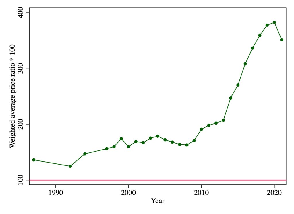
First, the domestic price of specific pharmaceuticals strictly exceeds the foreign price. According to a RAND study (Mulcahy et al. 2021), the average price of brand-name drugs in the United States is approximately 3.5 times the average price of those same drugs abroad. Even when the secret rebates and discounts manufacturers routinely offer their customers are taken into account, domestic prices are considerably higher than their foreign counterparts (House Ways and Means Committee Staff 2019).

Second, other high-income countries negotiate with manufacturers over the prices they charge. As the Council of Economic Advisers (2018) notes, “Most OECD nations employ price controls in an attempt to constrain the cost of novel biopharmaceutical products, e.g. through cost-effectiveness or reference pricing policies.”

Third, even the lower prices in Canada and Western Europe are far higher than the marginal cost of production—sometimes hundreds of times larger. For example, no price in Western Europe for a 12-week course of Sovaldi, one of several drugs to treat the hepatitis C virus (HCV), is below $40,000. And yet “a recent study estimated the cost of production of sofosbuvir [Sovaldi] to be U.S. $68-$136 for a 12-week course of treatment based on the same manufacturing methods used in the large-scale generic production of HIV/AIDS medicines (Hill et al. 2014), and its findings have not been challenged” (Iyengar et al. 2016). Other direct action antiviral (DAA) treatments for HCV (Epclusa, Harvoni, Mavyret, etc.) have similar costs of production (Hill et al. 2014).

The fourth stylized fact requires more discussion. Through their trade organization (the Pharmaceutical Research and Manufacturers of America, or PhRMA) and through “non-profit” organizations such as Partnership for Safe Medicines (PSM) which misleadingly appear to be independent, drug companies have spent millions of dollars warning that imported pharmaceuticals are dangerous because they may be counterfeits. Counterfeit pharmaceuticals are undeniably dangerous. But the actions of the manufacturers and PhRMA, often taken by the “independent” organizations they fund, make clear that consumer protection is a pretext; the real goal of the manufacturers is to protect the lucrative U.S. market from arbitrageurs acquiring the same goods from other high-income countries at a fraction of the price. Raising doubts about the safety of imported drugs follows a plan developed by a PR firm, Edelman, which PhRMA had retained. According to the Wall Street Journal (WSJ 2003), Edelman concluded on the basis of focus groups of people without drug-insurance coverage that safety, not legality, was their central concern when deciding whether to import their prescription drugs to save money. In response, PhRMA paid their “independent” organizations millions of dollars to publicize the dangers of drug importation. For example, according to Bloomberg (2019), PSM received $7.3 million in 2019 alone for this purpose. One such organization was the consulting firm of the former FBI Director Louis Freeh. Freeh reported that imports would “open a new, unregulated pipeline into the United States” despite the fact that none of the 16 states then proposing drug importation plans would have allowed imports from unregulated online pharmacies.1 Another such organization was the National Sheriffs Association. Basing their conclusions on Freeh’s report, sheriffs began appearing in hundreds of ads in the summer of 2019 imploring “the country’s leaders to reject proposals to import cheaper prescription drugs from other countries.” Robocalls in Florida even denounced a proposed state law claiming (without the slightest basis) that it “would legalize importing prescription drugs from China, which has a long history of producing counterfeit medications. . . ” As the Republican state representative who introduced Florida’s drug importation bill noted, it was “a good, old-fashioned scare campaign. Their real fear is this could have a significant impact on the profit margins of drug companies.”

In fact, importation from Canada will have only a minor effect on the profitability of the U.S. market since the population of Canada is 11.5% that of the United States. But the combined population of the other high-income countries with tightly regulated prescription drug markets is comparable to our own, and drug imports from them would devastate the drug companies’ most lucrative market. Such imports could be purchased by prescription holders themselves online or, in the rare circumstances when travel is feasible, in person.

Alternatively, prescription drugs could be imported by large commercial enterprises like Amazon, Costco, Sam’s Club, CVS, Walgreens, Rite Aid and sold to holders of prescriptions in person or online. All of these enterprises currently sell in the U.S. online (as well as in person). There is no reason to think importation from regulated outlets licensed in high-income countries are less safe than prescription drugs purchased in the U.S. As Michael Law, holder of the Canada Research Chair in Access to Medicines dryly observed: “People aren’t dying in the streets of Canada from unsafe medications” (Bloomberg 2019). They aren’t dying in the streets of the U.K., France, Germany, Switzerland, Australia, New Zealand, and Japan, either. In reality, the FDA has never reported a death or adverse reaction suffered by any patient in the U.S. who has personally filled his valid prescription online or in person from a pharmacy licensed in another high-income country.

Finally, if drug manufacturers were genuinely concerned about the safety of imports, they would not have sought to eradicate an organization like PharmacyChecker.com, whose mission includes protecting consumers from counterfeit drugs by identifying pharmacies licensed in high-income countries from which they can safely fill their prescriptions at a lower cost.2 Groups like PSM would instead either have financially supported such private certification organizations or would have advocated that their role be taken over by a government agency like the FDA.3 In summary, the fourth stylized fact is that drug manufacturers annually spend millions of dollars blurring the distinction between dangerous counterfeit drugs and safe drugs sold by pharmacies licensed in other high-income countries.4

Every model previously proposed to analyze the international drug market is inconsistent with at least one prominent feature of this market. For instance, Berndt (2002, 2007), Danzon (1997) and others regard the international pharmaceutical market as an example of third-degree price discrimination (Robinson 1933). While this model predicts prices in the two markets will differ, with the lower price exceeding the marginal cost of production, it assumes that prices in the foreign market are set by the monopolist without any negotiation.5 Moreover, these models of price discrimination ignore the massive investments manufacturers make in order to deter arbitrage. Hence, these models violate stylized facts (2) and (4).

Pecorino (2002) was the first to recognize that the foreign price is the result of bargaining. He assumes that a single manufacturer sells in the U.S. market at the monopoly price and in the foreign market at a price determined by the Nash bargaining model. Pecorino considers a regime where there is neither actual nor threatened arbitrage. Hence, there is no linkage between the two markets. The manufacturer always sells at the monopoly price in the U.S. If the foreign government has some bargaining power, the manufacturer sells at a strictly lower, negotiated price in the foreign market; unless the foreign government has all the bargaining power, the negotiated foreign price will exceed the constant marginal cost of production. Thus, Pecorino’s model is consistent with the first three stylized facts. However, it cannot explain stylized fact (4). Why spend millions of dollars to deter imports if there is no threat of imports?

Like Pecorino (2002), Egan and Philipson (2013) envision government bargaining down prices. They emphasize that paying for R&D through drug prices is costly to each country but the innovations that may result benefit all countries. Hence, there is a public goods problem and free-riding limits aggregate spending on R&D: “a small European country has no access-innovation trade-off in its pricing; it will have low reimbursements because it does not affect world returns and sees the same innovations regardless of its reimbursement policy.” Hence, it will bargain the price down close to the marginal cost of production: “the smaller the share of world demand and supply a country makes up, the less that government will mark up prices above cost to promote innovation.” Egan and Philipson’s theory takes no account of firm behavior. In neglecting firm behavior, they imply that firms will accept any price—as long as it is above their short-run marginal cost.

Egan and Philipson also take no account of arbitrageur behavior. Since the implied price differentials under their theory may be enormous, they presumably assume that arbitrage can never occur regardless of prices. In that case, there should be no spending by firms to raise the cost of consumer arbitrage. Thus, their theory violates stylized facts (3) and (4).

Like Egan and Philipson (2013), the Council of Economic Advisors (2018) discusses a case where the manufacturers and foreign governments negotiate over the foreign price but again there is no threat of arbitrage. Unlike Pecorino (2002), the Council assumes the foreign government faces $n \geq 1$ manufacturers and has all the bargaining power; it is as if the government simultaneously proposes a price to these $n$ manufacturers on a take-it-or-leave basis: “. . . in price negotiations with manufacturers, foreign governments with centralized pricing exploit the fact that once a drug is already produced, the firm is always better off selling at a price above the marginal cost of production and making a profit, regardless of how small, than not selling at all. Thus, the foreign government can insist on a price that covers the marginal production cost—but not the far greater sunk costs from years of research and development—and firms will continue to sell to that country” (CEA 2018, 15; 141 emphasis added).6 The prediction that the foreign price must equal marginal cost conflicts with stylized fact (3). As with Pecorino (2002), this model is also inconsistent with stylized fact (4) since there is no need to spend massively to deter arbitrage when there is no threat of arbitrage.

The situation where there is a single manufacturer and the foreign negotiator has all the bargaining power is a special case of both the Council’s and Pecorino’s models. Both predict a foreign price equal to the marginal cost of production. But imagine what would really happen if producers of drugs to cure hepatitis C sold them for $65,000 per cure (their current price) in the U.S. market and for $140 (marginal cost) in the market of other high-income countries. Since the market of the other high-income countries, taken as a group, is so large, arbitrage into the U.S. would occur on a massive scale. Demand at the $65,000 price would plummet, creating an incentive for the manufacturers to narrow the price differential between the two markets below what these models predict.7

Ganslandt and Maskus (2004) were the first to recognize that pricing to deter arbitrage might be advantageous to a manufacturer. They sketch a model where a single manufacturer with zero marginal cost can sell the same product in the foreign market at a price cap set exogenously and in the home market at a price of its choosing. If the difference between the two prices strictly exceeds an exogenous threshold, arbitrage is “accommodated” and if the price difference is no larger than that threshold, arbitrage is deterred. In their model, the foreign price cap is exogenous, conflicting with stylized fact (2). There is also no spending to scare consumers, a violation of stylized fact (4).

The contribution of the current paper is to provide a tractable model of the international pharmaceutical market for some therapeutic class of drugs (blood thinners, hypertension drugs, hepatitis C direct action antivirals, etc.) consistent with all four prominent characteristics of that market. The model combines the feature of arbitrage deterrence sketched in Ganslandt and Maskus (2004) with the bargaining model outlined in CEA (2018). In particular, we assume that if the difference between the high U.S. retail price and the low foreign retail price is sufficiently great, massive arbitrage would occur. We maintain all of the other assumptions of the Council. In particular, we continue to assume that a single negotiator bargains with $n \geq 1$ manufacturers on behalf of all the foreign governments and that it proposes the price it is willing to pay on a take-it-or-leave-it basis. In this way, we show how a single change in assumption alters the prediction of the Council.

It is common to consider the two extremes: either arbitrage is illegal, the markets are unconnected, and the domestic and foreign prices are independent of each other; or arbitrage is legal, the markets are perfectly connected, and the domestic and foreign prices coincide.8 However, there is a neglected intermediate case where importing prescription drugs is illegal, but nonetheless the markets are connected. Banning pharmaceutical imports does not eliminate importation; it merely makes engaging in it more costly. Massive arbitrage would still occur if the price difference were sufficiently great. Our formulation permits consideration not only of the two extremes but also of this intermediate case where the threat of arbitrage leads manufacturers to reject a negotiated foreign price any closer to the marginal cost of production.

In the equilibrium of this intermediate case, the difference in prices that emerges is just small enough to deter massive arbitrage. Only inframarginal buyers with unusually low thresholds would still purchase from foreign pharmacies. Recent empirical findings (Hong et al. 2020) are consistent with this prediction: “The findings suggest that patients are not using prescription purchases outside the U.S. to meet their medication needs.” In particular, according to this study based on 61,238 adults taking prescription medicines, a mere 1.5% of U.S. adults purchasing prescription medications bought them abroad to save money.9 Hence, the pharmaceutical industry’s intensive (and expensive) campaign to scare and confuse potential importers has succeeded. It has deterred the 98.5% of U.S. purchasers from reaping the huge savings available had they filled their prescriptions at the same licensed pharmacies that patients in other high-income countries routinely utilize to treat the same illnesses. A welfare implication of the situation modelled should be emphasized. Policies that benefit U.S. consumers do not do so by stimulating more arbitrage. The benefits arise instead because these policies motivate profit-maximizing manufacturers to lower domestic prices to deter arbitrage.10

It is important to distinguish two kinds of arbitrage that can be triggered if price differences between markets are sufficiently large: (1) personal arbitrage by patients seeking the least expensive cure for their illness and (2) commercial arbitrage by firms that buy and then resell whatever quantity of cures maximizes their profits. While both forms of arbitrage are illegal, personal arbitrage for own use has never been prosecuted. On the other hand, the law against commercial arbitrage is strictly enforced.

That may change. Bills have been proposed to legalize both kinds of arbitrage: “The Safe and Affordable Drugs from Canada Act of 2021” (S. 259), introduced by Senator Klobuchar on February 4, 2021 focuses on personal imports from Canada. It removes the discretion the FDA currently has to intercept personal imports from Canada. It explicitly requires that such imports be allowed if the dispensing pharmacy is licensed in Canada and provides the medication using a valid prescription from a physician licensed in any U.S. State.

“The Affordable and Safe Prescription Drug Importation Act” (S.920), introduced by Senator Sanders on March 23, 2021, is more sweeping. It allows individuals to use a licensed foreign pharmacy in any country to fill a U.S.-issued prescription for personal use (up to a 90-day supply), requires HHS to issue regulations that permit commercial importation from Canada and, at HHS’s discretion after a two year delay, to permit commercial importation from the OECD and other countries. Finally it imposes criminal penalties for online websites that sell counterfeit drugs or dispense drugs without a required prescription. Thus, in future years the importing may be done by Amazon Pharmacy or Costco.11

We proceed as follows. In Section 2, we introduce our model of personal importation, show that it has a unique subgame-perfect equilibrium, and that despite our assumption that the foreign negotiator has all the bargaining power, he is unable to negotiate the price down to the marginal cost of production. In Section 3, we show how the same framework can be used to determine domestic and foreign prices if the threat comes instead from commercial arbitrage. Section 4 concludes the paper.

Personal Arbitrage

Personal arbitrage typically occurs when a patient with a valid U.S. prescription orders online from a pharmacy which may be as close as Canada or as far away as New Zealand. Many foreign pharmacies receiving a prescription from an American patient routinely fill the order with the version of that drug approved in their own country. In countries where pharmacists are required to receive a prescription from a local doctor, the current practice is for the local doctor to review the U.S. prescription and the patient history and write a new prescription (“cosigning”) for the foreign version of the medication. Although importing prescription drugs into the United States for own use is technically illegal, no one has ever been prosecuted for this “crime,” which is victimless.

Although it is less common than online purchasing (Levitt, 2015), some patients have traveled to a foreign country such as Canada or a member of the EU, filled their prescriptions, and returned home.12 Enforcement then seems even more problematic since a patient can always disguise the drug purchased abroad by putting it in empty bottles (either from old prescriptions or over-the-counter medications). Even if the authorities were capable of stopping personal arbitrage, it seems unwise politically to separate a grandmother from the only medication she can afford to treat her cancer.

We hypothesize that if patients with valid prescriptions could save enough money by purchasing from foreign pharmacies instead of from American pharmacies, there would be massive personal arbitrage. We denote the threshold difference in retail prices as $\Delta$. Like Ganslandt and Maskus (2004), we assume this threshold is exogenous.13

Let $p^{U}$ denote the price the manufacturers charge wholesalers in the United States and $p^{N}$ denote the price they charge wholesalers for the same medication abroad. Let $\tau_{w}>1$ denote the exogenous markup of wholesalers, so that they charge local pharmacies at home and abroad $\tau_{w} p^{U}$ and $\tau_{w}p^{N}$, respectively. Let $\tau \geq \tau_{w}$ denote the exogenous combined markup of wholesalers and retailers at home and abroad, so that the retail prices are, respectively, $\tau p^{U}$ and $\tau p^{N}$. We assume that massive personal arbitrage will occur if $\tau(p^{U}-p^{N})>\Delta$ and none (apart from inframarginal imports) will occur if $\tau(p^{U}-p^{N})\leq \Delta$.

The U.S. government can lower $\Delta$ exogenously by scaling down misleading FDA warnings about the riskiness of taking medications routinely dispensed by licensed pharmacies in other high income countries; legalizing personal arbitrage would have similar effects, since it would reassure U.S. consumers about the safety of prescriptions filled at such pharmacies.

We consider $n \geq 1$ manufacturers, each producing one therapeutically equivalent, branded drug (such as the DAAs to cure hepatitis C, the vaccines to prevent Covid-19, blood thinners, hypertension drugs, etc.) at zero marginal cost and selling them at a market-determined price in the United States and at a negotiated price ceiling in the EU and Canada. The cap is set in the following game between the $n$ manufacturers and the negotiator. At the time of this bargaining, the R&D cost for developing the drug is a sunk cost.

Description of the Bargaining Game of Perfect Information

In this subsection, we describe the price negotiations between the agent representing the foreign governments and the $n$ manufacturers. Since none of the bargaining games in the literature seemed appropriate for our purposes, we constructed a tractable noncooperative bargaining game.14 The subgame-perfect equilibrium of this game is unique, intuitive, and amenable to graphical comparative-static analysis.15

We envision the following game. A single negotiator specifies a discounted price $p^{N}$ per cure at which to purchase medication for each of the (exogenous) $Q^{N}$ sufferers of a specific malady (such as hepatitis C).16 The negotiator proposes this price sequentially to each of the $n \geq 1$ drug manufacturers. If $k$ of them accept his proposal, he orders $Q^{N}/k$ from each of them. Those rejecting the negotiator’s proposal produce and sell only in the unnegotiated (U.S.) market. Those accepting it sell not only in the U.S. market but also in the foreign market. In the next subsection, we deduce the unique subgame-perfect equilibrium of this bargaining game.17

Intuitively, manufacturers benefit if they accept the negotiator’s proposal since each manufacturer can then sell in the foreign market a drug that is costless to produce. On the other hand, every manufacturer also incurs a cost in the U.S. market if any of them accepts the negotiator’s proposal because of actual or potential arbitrage. As a simplification, we assume that if arbitrage were to occur, all $Q^N$ cures obtained by the foreign negotiator would flow into the U.S. We relax this assumption at the end of the section.

If $Q^{N}$ were small relative to the size of the U.S. market, importation would be insignificant and the manufacturers would accommodate arbitrage by playing Cournot using a demand curve shifted inward slightly by the negligible amount $Q^{N}$. That is, manufacturers would sell in the U.S. market to the vast majority of patients lacking the good fortune to have acquired the $Q^{N}$ imports. However, since pharmaceuticals would be imported not only from Canada but from all the other OECD countries, $Q^{N}$ is large relative to the U.S. market and manufacturers would find arbitrage deterrence more profitable than accommodation.18 Hence, the consequence of any manufacturer accepting the negotiator’s proposal is a retail price in the U.S. market of at most $\Delta$ more than the retail price abroad.

Given the extremely low marginal costs of production for most drugs (recall the costs reported in Section 1), we assume that producing additional cures is costless.19 In addition, we assume that the drugs in this therapeutic class are perfect substitutes and therefore sell at the same price. Throughout, we assume that domestic retail demand, denoted $D(\cdot)$, depends on the retail price $p=\tau p^{U}$ and satisfies the following conditions: (1) $D(0)$ is finite, (2) $pD(p)$ is strictly concave and achieves a maximum at $p^{*}>\Delta>0$, and (3) there is a unique Cournot equilibrium in the game where the $n$ manufacturers sell simultaneously in the U.S. market and earn $p^{Cournot}/\tau=p^{U}$ per cure.

Table 1. Payoffs to manufacturer i

The negotiator approaches each manufacturer in sequence and proposes to pay $p^{N}$ per cure for $\frac{Q^{N}}{k}$ cures, where $k=1, \ldots, n$ is the number of manufacturers that ultimately accept. After the last manufacturer makes his decision, payoffs in the bargaining game are collected. The payoffs result from the subsequent simultaneous sales by the $n$ manufacturers.

If every manufacturer rejects the negotiator’s proposal, then each of the n manufacturers sells only in the U.S. market and receives an equal share of Cournot retail profits deflated by the markup factor ($\tau$). If $k \geq 1$ manufacturers accept the negotiator’s proposal but $\tau p^{N}+\Delta > p^{Cournot}$, then each of those accepting the proposal earns $p^{N}Q^{N}/k$ in the foreign market while those rejecting it earn nothing there. The U.S. retail price is $p^{Cournot}$, which is insufficient to compensate arbitrageurs given the high cost ($\tau p^{N}+\Delta$) of acquiring foreign drugs. No arbitrage occurs. Every manufacturer therefore again earns in the U.S. market an equal share of Cournot profits deflated by the markup factor ($\tau$).

If $\tau p^{N}+\Delta<p^{Cournot}$ and at least one of manufacturers accepts the negotiator’s proposal ($k \geq 1$), then each of the $k$ manufacturers earns $p^{N}Q^{N}/k$ in the foreign market while the $n-k$ others earn nothing in that market. In the U.S. market, however, a price of $p^{Cournot}$ would attract massive arbitrage. To deter it, limit pricing occurs instead. Each manufacturer sells enough more than its Cournot output in the U.S. market that the U.S. retail price ($\tau p^{U}$) drops to $\tau p^{N}+\Delta$. No manufacturer would unilaterally sell less than $D(\tau p^{N}+\Delta)/n$, under a weak condition insuring that arbitrage deterrence occurs in equilibrium. Nor would any manufacturer unilaterally sell more than this quantity since, with every firm producing an output exceeding the Cournot level, selling more would drive the U.S. retail price further away from the revenue-maximizing level. Hence, if any manufacturer accepts the proposal, the retail price in the U.S. market would be $\tau p^{N}+\Delta$, but no importing would occur.

In Table 1, we list for any proposed $p^{N}$ the payoffs manufacturer i would receive in this bargaining game. These payoffs depend not only on his accept-reject decision but on those of the $n-1$ other manufacturers.

The Unique Subgame-Perfect Equilibrium in the Bargaining Game

We now consider how each manufacturer in the sequence would respond to any proposed $p^{N}$. Each manufacturer in the sequence would find himself in one of two situations: either (1) some firm earlier in the sequence had already accepted the negotiator’s proposed price $p^{N}$ or (2) no previous manufacturer had accepted the proposed price. We work backwards, considering first the optimal choice of the final manufacturer in the sequence.

We consider two cases. In the first case, the proposed price satisfies:

\[p^{N}Q^{N}+\frac{(\tau p^{N}+\Delta)D(\tau p^{N}+\Delta)}{\tau n}>\frac{\pi^{Cournot}}{\tau n}\] (1)

If someone previously had accepted the proposal, the final manufacturer would accept as well. For, even if he rejected the proposal, there would still be $Q^{N}$ cures that would 338 flood the U.S. market unless arbitrage was deterred. By accepting and selling in the foreign 339 market, he would earn revenue additional to his domestic sales.

If no one had previously accepted, the final manufacturer would strictly prefer to accept. For by being the only manufacturer to accept, he would earn $p^{N}Q^{N}$ in the foreign market plus $\frac{(\tau p^{N}+\Delta)D(\tau p^{N}+\Delta)}{\tau n}$ in the domestic market, which according to inequality (9) strictly exceeds $\pi^{Cournot}/\tau n$, the revenue he would earn if he rejected the negotiator’s proposal. So the final manufacturer would accept such a proposal even if no firm prior to him had accepted it.

Turning now to the optimal decision of the penultimate manufacturer, he would accept the proposal if any previous manufacturer had accepted; for, there would then be the arbitrage threat of the $Q^{N}$ cures in the foreign market whether he accepted or rejected the proposal, and he would strictly increase his revenue by also selling in the foreign market. If no previous manufacturer had accepted the proposal, the penultimate manufacturer would anticipate that if he rejected it as well, the final manufacturer would nonetheless accept it since that is his best reply in that situation. Thus, the penultimate manufacturer recognizes that there would be $Q^{N}$ cures in the foreign market to be deterred from flooding the U.S. market regardless of his decision; he accepts and strictly increases his revenue by $p^{N}Q^{N}$ / 2 since he would divide the foreign market with the final manufacturer.

Any previous manufacturer would behave in the same way. If someone had previously accepted, he would accept to get some share of the foreign market. If no one had previously accepted and he also rejected, he would anticipate that every subsequent manufacturer would best-reply by accepting the negotiator’s proposal. Hence, he would anticipate that regardless of what he did the $Q^{N}$ cures would still loom over the U.S. market and that by accepting he would get an additional $p^{N}Q^{N}/(1+z)$ in revenue, where $z$ is the number of manufacturers who move after him.

Suppose instead the proposed $p^{N}$ satisfies the following inequality:

\[p^{N}Q^{N}+\frac{(\tau p^{N}+\Delta)D(\tau p^{N}+\Delta)}{\tau n}<\frac{\pi^{Cournot}}{\tau n}\] (2)

As before, the final manufacturer and every predecessor would accept the proposed price if any previous manufacturer had previously accepted it. Suppose, however, that the final manufacturer observed that no one had previously accepted the proposed price. If he accepted it, inequality (2) indicates that he would be strictly worse off than if he joined his predecessors in rejecting the proposal and competed only in the U.S. market; for if none of the $n$ manufacturers sells in the foreign market, there would be no need to deter arbitrage and he would earn his share of Cournot profits deflated by the markup $\tau$. Now consider the penultimate manufacturer. If he observed that no one had previously accepted the negotiator’s proposal, then—anticipating that the final manufacturer would reject it if he did, he would reject $p^{N}$ as being too low. Indeed, every prior manufacturer would be in the same position. If he rejected the proposal, every subsequent manufacturer would do so as well and there would be no threat of imports flooding the U.S. market. The $n$ firms would each get a share of the Cournot profits in the U.S. market.

\[p^{N}Q^{N}+\frac{(\tau p^{N}+\Delta)D(\tau p^{N}+\Delta)}{\tau n}=\frac{\pi^{Cournot}(n)}{\tau n}\] (3)

Since the foreign negotiator wants to purchase $Q^{N}$ cures at the lowest price, he would propose a price just above $\bf{p}^{N}$. In the play of the game, every manufacturer accepts proposal ${\bf p}^{N}$, and each firm receives $1/n^{th}$ of the additional $Q^{N}$ sales. The retail price in the U.S. market falls to $\tau p^{U}=\tau p^{N}+\Delta$, just low enough to deter arbitrage. The $n$ manufacturers sell $Q^{N}$ cures in the negotiated market and $D(\tau {\bf p}^{N}+\Delta)$ in the unnegotiated market.

If $n=1$, the right-hand side of equation (2.3) is the monopoly profit the firm would receive if it sold only in the U.S. market and the left-hand side is the profit it would receive from selling to wholesalers at price $p^{N}$ in the foreign market and at price $p^{N}+\Delta/\tau$ in the U.S. market, the highest price it can charge without triggering arbitrage. The equality of the two sides indicates that the foreign negotiator drives the foreign price ($p^{N}$) down so that the monopolist earns no more profit selling in both markets than it would receive selling only in the U.S. market. If $n>1$, the payoff on the right-hand side is the profit per firm every firm would earn if it sold only in the U.S. market. As for the left-hand side, it is what any one firm conjectures it would earn if it broke ranks with the other $n-1$ firms and accepted the negotiator’s proposal of $p^{N}$ instead of rejecting it. The equality of the two sides indicates that the foreign negotiator bargains the price down as far as he can; it would be in the self-interest of each manufacturer to reject his price proposal if it were any lower.20

It is helpful to rearrange equation (3) as follows:

\[(\tau p^{N}+\Delta)D(\tau p^{N}+\Delta)=\pi^{Cournot}(n)-\tau np^{N}Q^{N}\] (4)

The right-hand side is a decreasing linear function of $p^{N}$ with vertical intercept $\pi^{\mbox{ Cournot }}(n)$ and slope $-\tau nQ^{N}<0$. The left-hand side is a strictly concave function with vertical intercept $\Delta D(\Delta) \geq 0$. Given our assumptions about the function $D(\cdot)$, domestic total retail revenue $(\tau p^{N}+\Delta)D(\tau p^{N}+\Delta)$ is strictly increasing at $p^{N}=0$.

Since Cournot profit is strictly smaller than monopoly profit (for $n=2,\ldots$), the vertical intercept of the line is strictly smaller than the peak of the concave profit function. There are two possible cases. In the first case, $\Delta \leq p^{Cournot}$, the domestic and foreign markets are “connected” and ${\bf p}^{U}={\bf p}^{N}+\Delta/\tau$; in the second case, $\Delta > p^{Cournot}$, the two markets are “unconnected” and $p^{N}=0$ (marginal cost) while ${\bf p}^{U}=p^{Cournot}/\tau$. The first case (respectively, the second case) arises if the vertical intercept of the single-peaked function lies below (resp. above) the vertical intercept of the downward-sloping line. In the two cases,

\[{\bf p}^{U}=\min \left({\bf p}^{N}+\Delta/\tau, p^{Cournot}\right/\tau)\]

In the connected case, the horizontal component of the point of intersection is the manufacturer’s foreign price (${\bf p}^{N}$), and the vertical component is the total retail revenue in 402 the domestic market. In the unconnected case, the negotiated manufacturer’s price abroad equals the marginal production cost (assumed, for simplicity, to be zero), and the retail 404 price in the U.S. market is the Cournot price. We depict the determination of ${\bf p}^{N}$ in Figure (1):

Figure 1. Determination of the foreign price when there is a threat of personal arbitrage.

In deriving the equilibrium, we assumed as a simplification that if the price differential were large enough to make personal arbitrage attractive, all of the $Q^{N}$ cures sold in the foreign market would be imported into the U.S. We conclude this section by showing that such an extreme assumption is not necessary for arbitrage deterrence to occur in the equilibrium.

Suppose some firm unilaterally deviated from the proposed arbitrage deterrence equilibrium, by reducing his sales in the domestic market and driving the price up to $p^{U}>{\bf p}^{N}+\Delta/\tau$. Suppose that as a result, there were only $\theta Q^{N}$ cures imported for own use, where $\theta \in (0,1)$. This unilateral deviation would not affect the deviator’s revenue in the foreign market. He would still sell $Q^{N}/n$ cures at the price $\tau {\bf p}^{N}:\; \theta Q^{N}/n$ to Americans importing for own use and $(1-\theta)Q^{N}/n$ to foreigners. However, the unilateral deviation would change the deviator’s revenue in the domestic market by:

\[p^{U}\left(D(\tau p^{U})-\frac{n-1}{n}D(\tau {\bf p}^{N}+\Delta)-\theta Q^{N}\right)-\frac{(\tau {\bf p}^{N}+\Delta)}{\tau n}D(\tau {\bf p}^{N}+\Delta)\] (5)

where $p^{U} \geq {\bf p}^{N}+\Delta/\tau$.

The second term in (5) is the revenue the deviator receives in the equilibrium from sales in the U.S. market. The first term is the revenue the deviator would get from unilaterally reducing his U.S. sales enough to drive the price up to $p^{U}$. The second factor of the first term is the amount he would have to sell to accomplish this price increase—the aggregate demand in the U.S. minus the sum of personal imports and the sales from the $n-1$ non-deviators, conjectured to be unchanged.

If the foreign country was small (e.g. Monaco) or θ was small, $\theta Q^{N}$ would be negligible and (2.5) reduces to zero when $p^{U}={\bf p}^{N}+\Delta/\tau$. Since in the equilibrium, every firm is selling more than his Cournot output, even a marginal output contraction by the deviator would make his deviation strictly profitable. In this case, no equilibrium with arbitrage deterrence can exist. On the other hand, if $\theta Q^{N}$ were sufficiently large, the unchanged sales in the U.S. of the $n-1$ rivals plus the large personal imports ($\theta Q^{N}$) of the Americans might virtually satisfy U.S. market demand at ${\bf p}^{N}+\Delta/\tau$. In that case, the deviator’s sales would be meager and his unilateral deviation would be massively unprofitable. Consider any $Q^{N}$ large enough that when $\theta=1$, the most profitable deviation results in a strict loss. Since the deviator’s revenue in the domestic market from his most profitable deviation is continuous in $\theta$, his deviation will also result in a strict loss for any $\theta \in (\theta^{*},1)$ where $\theta^{*}$ is the unique root of the maximized value of the expression in (5).21

Commercial Arbitrage

We have postponed discussion of commercial importation until now because (1) the analysis parallels that of personal arbitrage and (2) the ban on commercial importation is currently strictly enforced.

Since importers must pay a foreign wholesaler as much as local pharmacies pay it, importers must pay the wholesaler $\tau_{w}p^{N}$ per unit. Assume the exogenous per-unit cost of importing is the same for all importers and denote it $\Delta^{c}$. Since the ban against commercial importation is currently strictly enforced, $\Delta^{c}$ is high ($\Delta^{c}>>\Delta$). But it will drop precipitously ($\Delta^{c}<<\Delta$) if Senator Sanders bill or a similar one becomes law.

There are three types of commercial importers: (1) dispensers like Amazon, CVS, or Costco which sell to U.S. prescription holders; (2) U.S. wholesalers which sell to U.S. pharmacies; and (3) U.S. arbitrageurs which sell to U.S. wholesalers. If the importer is a dispenser, it earns a per-unit profit of $\tau p^{U}-\tau p^{N}-\Delta^{c}$. If the importer is a U.S. wholesaler, it earns a per-unit profit of $\tau_{w}p^{U}-\tau_{w} p^{N}-\Delta^{c}$. If the importer is an arbitrageur, it earns a per-unit profit of $p^{U}-\tau_{w}p^{N}-\Delta^{c}$. Since $\tau>\tau_{w}>1$, the largest per-unit profit would be earned by the dispensers. Hence, if the dispensers are deterred, so too will the other two types of commercial importers.

To summarize, commercial importation is deterred if and only if:

\[\tau p^{U}\leq \tau_{w}p^{N}+\Delta^{c}\] (6)

Previously, it was shown that personal importation is deterred if and only if:

\[\tau p^{U} \leq \tau p^{N}+\Delta\] (7)

We also concluded that the retail price in the U.S. will be no higher with an arbitrage threat than without one:

\[\tau p^{U} \leq p^{Cournot}\] (8)

Finally, the foreign negotiator’s offer will be accepted if and only if:

\[np^{N}Q^{N}+p^{U}D(\tau p^{U}) \geq \frac{\pi^{Cournot}}{\tau}\] (9)

The lowest price the foreign negotiator can secure must be acceptable to the firms but without triggering either type of arbitrage.

In Figure 2, the foreign manufacturers’ price is on the horizontal axis and the U.S. manufacturers’ price is on the vertical axis. The personal arbitrage constraint is depicted as a line sloping upward at 45 degrees with a vertical intercept of $\Delta/\tau$; the commercial arbitrage constraint is depicted as a line sloping upward at a flatter slope ($\tau_{w}/\tau <1$) with vertical intercept $\Delta^{c}/\tau$. No arbitrage occurs if the two manufacturers’ prices ($p^{N}, p^{U}$) lie on or below both arbitrage constraints. In addition, the manufacturers’ price in the U.S. cannot exceed $p^{Cournot}/\tau$. Hence, $p^{U}$ must satisfy $p^{U} \leq \min({p^{Cournot}; p^{N}+\Delta/\tau; \frac{\tau_{w}}{\tau} p^{N}+\Delta^{c}/\tau})$. Finally, the negotiator will restrict his attention to prices that are above the downward-sloping line since only they will be accepted. Such price satisfy inequality (9).

Figure 2. Even though the foreign negotiator has all the bargaining power, he cannot bargain the price down to marginal cost since proposals resulting in commercial or personal arbitrage are unacceptable to the firms.

In Figure 2, the shaded set of manufacturer prices ($p^{N},p^{U}$) defined by the intersection of the four inequalities is labeled the “Feasible Set.” In constructing the diagram, we have assumed that commercial arbitrage has been legalized and so $\Delta^{c}<\Delta$. As a result, the commercial arbitrage boundary lies below the personal arbitrage boundary—the reverse of what is currently the case. To avoid clutter, the foreign negotiator’s field of indifference curves is not depicted. However, each curve is a vertical line and lines further to the left are preferred by the foreign negotiator since he prefers to pay less for them $Q^{N}$ cures that he procures. The optimal choice of $p^{N}$ occurs at the intersection of the downward-sloping line and the lower of the two upward-sloping lines. Since we have assumed that commercial importation has been legalized, its constraint is the relevant one. Before legalization of commercial arbitrage, the personal arbitrage constraint would have been the relevant one and the best choice of $p^{N}$ would have been lower and $p^{U}$ would have been higher.

Any foreign price proposed by the negotiator strictly to the left of the downward-sloping locus would be rejected; any proposed price on it or to its right would be accepted. If the markets are connected, the equilibrium negotiated price is the smallest $p^{N}$ that (1) deters massive arbitrage but (2) is acceptable to the manufacturers. This occurs where the downward-sloping line intersects the lower upward-sloping line.

Policies that shift the downward-sloping locus against an unchanged upward-sloping locus will result in the manufacturers’ U.S. price and negotiated foreign price changing in the same direction. For example, increases in $Q^{N}$ will lower both the foreign price and the domestic price.22

Policies that shift the upward-sloping locus against an unchanged downward-sloping locus will result in the U.S. price and the negotiated foreign price changing in opposite directions. For example, lowering $\min(\Delta, \Delta^{c})$ would raise the manufacturers’ foreign price and lower the manufacturers’ U.S. price.

We can express revenue per firm (denoted $R$) in terms of exogenous variables and $p^{N}$.

\[R=\frac{pQ^{N}}{n}+\frac{p^{U}D(\tau p^{U})}{n}\] (10)

At the optimum, (9) will hold as an equality. Substituting the equality into (10), we conclude:23

\[R=\frac{\pi^{Cournot}}{n\tau}-\frac{(n-1)}{n}p^{N}Q^{N}\] (11)

If $\min(\Delta, \Delta^{c})$ decreases and consequently the foreign price increases, equation (11) implies that manufacturer revenue and hence variable profit will decrease.

Conclusion

In this paper, we identified four stylized facts about the international market in branded pharmaceuticals that seem undeniable. We then showed that no model in the literature explains these facts, and we constructed a new model consistent with them.

Central to this explanation is the effect on manufacturer pricing of the threat of massive personal arbitrage. Legislation is being considered which will lower the cost of importing whether for own use or for commercial resale. If enacted into law, this legislation will reduce U.S. drug prices and will lower the variable profits of pharmaceutical manufacturers. As has been emphasized by Egan and Philipson (2013), CEA (2018), Danzon (1997) and others, these profits are used in part to fund the massive fixed cost of drug innovation. The induced decrease in profits may, therefore, reduce innovation. However, the evidence that welfare will decline as a result is ambiguous. Lakadawalla (2018), in his thorough survey of the empirical work on this issue, concluded: “We have stressed the uncertainty surrounding the normative analysis of innovation investment. The question of whether innovation is too high or too low is a first-order—perhaps the first-order— policy question in the economics of the pharmaceutical industry. Yet, economists have not produced a definitive answer.”

If welfare turns out to decline because of reduced R&D in this industry, subsidizing innovation can restore the rate of innovation to its previous level. To me, asking sick people to finance drug innovation, which is of value not only at home but abroad, is ethically indefensible. The burden falls heaviest on sick Americans since our prices are by far the highest. People currently in good health should shoulder more of the burden. Increased subsidization, financed by general taxes at home and abroad is, in my view, a step in the right direction.

Funding: This research was funded by the Michigan Institute of Teaching and Research (MITRE).

Acknowledgments: Jim Adams stimulated my interest in this topic, and I am indebted to him for many useful discussions. I also wish to thank Yuan Chen, Yichuan Wang, and Haozhu Wang for their valuable research assistance and Rabah Amir, Andrew Daughety, Gérard Gaudet, Stephen LeRoy, Joshua Linn, Joseph Newhouse, Yesim Orhun, Charles Phelps, Jennifer Reinganum, Anna Schmidt, and Jon Sonstelie for comments on earlier drafts. I am indebted to Gabriel Levitt for clarifying the mechanics of personal arbitrage and for his continuing encouragement. I am particularly grateful to Mingyuan Zhang for his research assistance and to Marius Schwartz for his extensive comments on a previous draft.

Conflicts of Interest: The author declares no conflict of interest. MITRE had no role in (1) the design of the study, (2) the writing of the manuscript, or (3) the decision to publish the results.

Footnotes

1 All the quotations in this paragraph are from the investigative report in Bloomberg (2019).

2 For a discussion of the tactics used by “a network of other groups closely aligned with U.S. pharmaceutical companies. . . to drive PharmacyChecker off the Internet” see Stoltz 2019.

3 The FDA could undoubtedly scale up the surveillance and certification function performed by Pharmacy- Checker.com. Bate et al. (NBER 2013) established that drugs purchased from foreign pharmacies certified safe by PharmacyChecker.com are just as safe as drugs purchased from domestic, brick-and-mortar pharmacies. To detect counterfeits, Bate et al. (NBER 2013) used Raman spectrometry (Witkowski 2005), one of the techniques the FDA uses to distinguish bona fide medicine from counterfeits and adulterated pharmaceutical products.

4 Although PhRMA’s annual lobbying expenditures were $63 million in 2015, the most recent full year for which data are available, annual payments to patient advocacy groups was at least 80% higher! While some of these groups advocate for patients suffering from particular diseases, others “effectively supplement the work lobbyists perform, providing patients to testify on Capitol Hill and organizing letter-writing and social media campaigns that are beneficial to pharmaceutical companies. . . Notably, such groups have been silent or slow to complain about high or escalating prices, a prime concern of patients” (Kopp et al. 2018).

5 Malueg and Schwartz (1994) analyze third-degree price discrimination by a monopolist. Their motivation differed from mine since they were motivated by parallel imports to the U.S. from very low income countries.

6 The academic literature (Grossman and Lai 2008, 386 and Figure 1) also predicts that when re-imports are illegal, governments imposing price controls will bargain down to the marginal cost of production under the plausible assumption that these countries are not too sizable compared with the region that innovates.

7 What would happen in this situation? Our model predicts the arbitrage-deterring pair of prices which would emerge in the two markets for Pecorino’s special case of a single manufacturer as well as for the Council’s more general case of multiple manufacturers.

8 Pecorino calls these the “No Reimports Regime” (NR) and the “Reimport Regime,” respectively. These are essentially the same two extremes on which Grossman and Lai (2008) focus in their valuable article on parallel trade.

9 The study goes on to document the socioeconomic and demographic characteristics of these inframarginal buyers. Many of these outliers are desperately poor or lacking in insurance. We assume that they would continue buy abroad even if the price differential marginally narrowed.

10 The Congressional Budget Office (CBO 2004) concluded that policies to reduce the exogenous threshold, such as legalizing arbitrage or reducing misleading safety warnings, would confer little benefit on U.S. consumers. In reaching this conclusion, CBO disregarded potential reductions in domestic drug prices and confined its estimate of benefits to increases in imports from the European Union and Canada. Under this approach, CBO would have disregarded the policy-induced price changes in our model and, since these are accompanied by no changes in pharmaceutical imports, would have erroneously concluded that no policy change affects consumers.

11 The threat of imports from all OECD countries is vastly more important since they have a population which is 35 times that of Canada.

12 In a signed letter to the New York Times, a rheumatologist observed that “a patient could fly first class to Paris, stay at the Ritz, dine at a top Michelin restaurant, buy a one-year supply of Humira [a rheumatoid arthritis drug] at local prices in France, fly back home and finish with enough profit to hire a registered nurse to administer the injection every two weeks” (Hanauer 2019).

13 If the arbitrage threshold is a strictly increasing but kinked function of the spending of the manufacturers and PhRMA, then the associated marginal cost of increasing that threshold will have vertical segments. We assume that any policy interventions leave the threshold unchanged at the same vertical segment. We denote the threshold $\Delta$. The threshold is endogenized in Salant (2023).

14 The Nash Bargaining Solution, the Kalai-Smorodinsky Solution, Harsanyi’s Utilitarian Solution, Rawls’ Equal Increments Solution, etc. are cooperative; the most attractive noncooperative one (Rubinstein 1982) would limit us to a single manufacturer; generalizations of Rubinstein to $n \geq 1$ manufacturers have multiple subgame- perfect equilibria (see Suh and Wen and the references therein); and, although the model of Horn and Wolinsky (1988) has $n\geq 1$ manufacturers, each government negotiator is required to bargain exclusively with one exogenously designated manufacturer and is therefore unsuitable for our application.

15 We conduct an illustrative analysis when discussing Figure 2. For a more systematic comparative-static analysis, see Salant (2021).

16 Kyle et al. (2008) emphasize that in many European countries, regulations leave pharmacies and patients with no incentive to purchase cheaper offerings. Given that they are so insulated from prices, we assume that $Q^{N}$ is completely insensitive to price.

17 In footnote 20, we show that the same equilibrium arises if the manufacturers respond to the negotiator’s proposal simultaneously instead of sequentially.

18 See the discussion at the end of the section.

19 Ganslandt and Maskus (2004) make the same assumption.

20 To be precise, if the $n$ manufacturers respond simultaneously instead of sequentially to the negotiator’s proposal, there are two equilibria. There is a degenerate equilibrium where everyone accepts a proposed $p^{N}$ no matter how low it is. Rejecting the proposal unilaterally does not alter the need for arbitrage deterrence and merely reduces a manufacturer’s own revenue by $p^{N}Q^{N}/n$. This equilibrium has no counterpart in the subgame-perfect equilibrium of the sequential game. The more plausible equilibrium in the simultaneous- move game is the counterpart of the subgame-perfect equilibrium in the sequential game. It is an equilibrium in the simultaneous-move game for everyone to reject the proposed price ${\bf p}^{N}$ defined implicitly by inequality (2). For, each manufacturer would receive the payoff on the right-hand side of this inequality whereas if one player unilaterally deviated by accepting the proposal, he would receive the profit on the left-hand side. If $p^{N}$ is reduced, the left-hand side is even smaller while the right-hand side does not change. Hence, rejecting the proposal remains an equilibrium for any proposed price lower than ${\bf p}^{N}$ . If the proposed price instead satisfies inequality (9), however, this unilateral deviation is strictly profitable and rejection is no longer an equilibrium. What is the equilibrium in this case? Any proposed price higher than ${\bf p}^{N}$ will be accepted by the $n$ manufacturers; for, if any manufacturer unilaterally rejected the proposal, he would lose $p^{N}Q^{N}/n$ revenue from the foreign market. Hence, to obtain $Q^{N}$ cures at the lowest price, the negotiator would propose a price marginally above ${\bf p}^{N}$ and every manufacturer would accept the proposal. None of the $Q^{N}$ sold in the foreign market would be imported back to the U.S.

21 The envelope theorem implies that the maximized value of (5) strictly decreases in $\theta$; hence the root $\theta^{*}$ is unique.

22 If (9) holds as an equality, any increase in $Q^{N}$ would, for a fixed $p^{N}$ , raise the first term and necessitate a reduction in the second term in order to preserve the equality. This in turn requires lowering $p^{U}$.

23 The revenue formula we derive holds whichever upward-sloping arbitrage constraint is binding since the derivation does not involve either of these constraints; it relies only on the definition of revenue and the equation for the downward-sloping line. Note that when $n=1$ and the Cournot oligopoly reduces to a monopoly, (11) reduces to $\pi^{Cournot}/\tau$.

References

Bate, R., G.Z. Jin, and A. Mathur. 2013. “In Whom We Trust: The Role of Certification Agencies in Online Drug Markets.” NBER Working Paper 17955. Cambridge, MA: National Bureau of Economic Research.

Berndt, E. 2002. “Pharmaceuticals in U.S. Health Care: Determinants of Quantity and Price.” Journal of Economic Perspectives 16 (4): 45-66.

Berndt, E. 2007. “A Primer on the Economics of the Re-importation of Prescription Drugs.” Managerial and Decision Economics 28: 415-

Bloomberg. 2019. “Sheriffs’ Ads Slammed Drug Imports, and Big Pharma Helped Pay the Tab.”October 23. Accessed at https://www.bloomberg.com/news/features/2019-10-23/big-pharma-helped-fund-sheriffs-ad-blitz-against-drug-imports

CBO (Congressional Budget Office). 2004. “Would Prescription Drug Importation Reduce U.S. Drug Spending? ” Economic and Budget Issue Brief. Washington, DC: CBO.

CEA (Council of Economic Advisers). 2018. “Reforming Biopharmaceutical Pricing at Home and Abroad.” Washington, DC: Government Printing Office.

Danzon, P. 1997. “Price Discrimination for Pharmaceuticals: Welfare Effects in the U.S. and the EU.” International Journal of the Economics of Business 4 (3): 301-321.

Egan, M. and T. Philipson. 2013. “International Health Economics.” NBER Working Paper 19280.

Ganslandt, M. and K. Maskus. 2004. “Parallel Imports and the Pricing of Pharmaceutical Products: Evidence from the European Union.” Journal of Health Economics 23:1035-1057.

Grossman, Gene M., and Edwin L.-C. Lai. 2008. “Parallel Imports and Price Controls.” RAND Journal of Economics 39 (2): 378-402.

Hanauer, L. 2019. “Anger over Drug Prices in the U.S.” New York Times, March 2: A20.

Hill, A., S. Khoo, J. Fortunak, B. Simmons, and N. Ford. 2014. “Minimum Costs for Producing Hepatitis C Direct-Acting Antivirals for Use in Large-Scale Treatment Access Programs in Developing Countries.” Clinical Infectious Diseases 58 (7): 928-936.

Hong Y.R., J.M. Hincapie-Castillo, Z. Xie, R. Segal, and A.G. Mainous. 2020 “Socioeconomic and Demographic Characteristics of U.S. Adults Who Purchase Prescription Drugsfrom Other Countries.” JAMA Network Open, June 24; 3(6): e208968. doi:10.1001/jamanetworkopen.2020.8968: p.1-12.

Horn, H. and A. Wolinsky. 1988. “Bilateral Monopolies and the Incentives for Merger.” The Rand Journal, Autumn, 19 (3): 409-419.

House Ways and Means Committee. 2019. “A Painful Pill to Swallow: U.S. vs International Prescription Drug Prices.” September.

Iyengar, S., K. Tay-Teo, S. Vogler, P. Beyer, S. Wiktor, K. de Joncheere, and S. Hill. 2016. “Prices, Costs, and Affordability of New Medicines for Hepatitis C in 30 Countries: An Economic Analysis.” PLOS Medicine 13 (5): 1-22.

Kopp, E., S. Lupkin, and E. Lucas. 2018.“Patient Advocacy Groups Take in Millions from Drugmakers. Is there a Payback?”Kaiser Health News. April 6. Accessed at https://khn.org/news/patient-advocacy-groups-take-in-millions-from-drugmakers-is-there-a-payback

Kyle, M., J. Allsbrook., and K. Schulman. 2008. “Does Re-importation Reduce Price Differences for Prescription Drugs? Lessons from the European Union.” Health Services Research 43 (4): 1308-1324.

Lakdawalla, D.. 2018. “Economics of the Pharmaceutical Industry.” Journal of Economic Literature 56 (2): 397-449.

Levitt, G. 2015. “Online Pharmacies, Personal Drug Importation and Public Health: Ill-Considered Enforcement Prevents Access to Safe and Affordable Medication.” Prepared for the Senate Committee on Health, Education, Labor and Pensions and the House Committee on Energy and Commerce.

Malueg, D., and M. Schwartz. 1994. “Parallel Imports, Demand Dispersion, and International Price Discrimination ” Journal of International Economics 37: 167-195.

Mulcahy, A., C. Whaley, M. Tebeka, D. Schwam, N. Edenfield, and A. Becerra-Ornelas. 2021. “International Prescription Drug Price Comparisons: Current Empirical Estimates and Comparisons to Previous Studies.” Rand Research Report RR2956.

Pecorino, P. 2002. “Should the U.S. Allow Prescription Drug Reimports from Canada?” Journal of Health Economics 21: 699-708.

Robinson, J. 1933.“Economics of Imperfect Competition.” London: Macmillan.

Rubinstein, A. 1982. “Perfect Equilibrium in a Bargaining Model.”Econometrica, 50:97-110.

Salant, S. 2021. “Arbitrage Deterrence: A Theory of International Drug Pricing.” RFF Working Paper 21-07.

Salant, S. 2023. “Spending and Pricing by a Monopolist to Deter Arbitrage.” Working Paper.

Shepherd, J. 2018. “Consolidation and Innovation in the Pharmaceutical Industry: The Role of Mergers and Acquisitions in the Current Innovation Ecosystem.” Journal of Health Care Law and Policy 21 (1): article 2.

Stoltz, M. 2019. “Suit Against Pharmacy Groups Uses Antitrust as a Weapon Against Unaccountable Online Censorship. ”Electronic Frontier Foundation. September 3.

Suh, S and Wen Quan. 2003. “Multi-Agent Bilateral Bargaining and the Nash Bargaining Solution” Journal of Mathematical Economics, Elsevier, vol. 42(1), pages 61-73.

Wall Street Journal. 2003. “Drug Companies Cry ‘Danger’ Over Imports.” September 22. Accessed at https://www.wsj.com/articles/SB106418061476794700.

Witkowski, Mark R. 2005. “The Use of Raman Spectroscopy in the Detection of Counterfeit and Adulterated Pharmaceutical Products.” American Pharmaceutical Review 8 (1): 645 56-62.

Benedic N. Ippolito, American Enterprise Institute, and Joseph F. Levy, Johns Hopkins Bloomberg School of Public Health

Contact: jlevy@jhu.edu

Abstract

What is the message? This paper explores whether the pricing of drugs relative to their clinical value affects insurance coverage and usage for drugs under Medicare Part D. The authors find that lower generic prices stimulate both greater use and more generous insurance coverage. However, for branded drugs they find no relationship for either coverage or use based on variation across drugs in their cost effectiveness, as estimated by the Institute for Clinical and Economic Review (ICER)

What is the evidence? An analysis of pharmacy-dispensed brand drugs without generic competition in the Medicare Part D market in 2022, with a particular emphasis on drugs which also have external value-based pricing estimates from the Institute for Clinical and Economic Review (ICER).

Timeline: Submitted: June 10, 2023; accepted after review Sept. 1, 2023.

Cite as: Benedic Ippolito, Joseph Levy. 2023. Drug Pricing Decisions and Insurance Coverage: Evidence from Medicare Part D. Health Management, Policy and Innovation (www.HMPI.org), Volume 8, Issue 2.

Download PDF

Introduction

Brand drugmakers have discretion over the prices of their products. These decisions have attracted significant attention, with many U.S. policymakers arguing that prices are too high relative to external benchmarks or estimated measures of clinical value. However, while drugmakers effectively set prices unilaterally, these decisions can trigger responses from purchasers that affect the quantity sold. In this paper, we explore this dynamic by investigating whether the pricing of drugs, relative to estimates of clinical value, affect the coverage and utilization of branded drugs in Medicare Part D.

In a simplified framework, an insurer that is willing to cover drugs priced well above their value to patients will generate premiums that are unattractively high relative to an insurer that is more judicious in coverage. Of course, an insurer need not passively cover drugs independent of their price. Instead, they have a number of tools that can impede beneficiaries’ access to such products. Perhaps most directly, a drug’s price can influence an insurer’s decision to cover a drug or not. Even conditional on coverage, insurers can impose differential levels of utilization management tools which have first-order effects on utilization. For example, applying prior authorization to a covered product reduces utilization of a drug by nearly 27 percent in Part D (Brot-Goldberg et al., 2023). Further, they can increase cost sharing for a given product or use coinsurance to make the out-of-pocket spending for beneficiaries a direct function of the (list) price of the drug.

We investigate how insurers within Medicare Part D choose to cover drugs with differential pricing strategies. Specifically, we ask whether drugs with particularly high prices, relative to an estimate of their clinical value, are covered at lower rates or subject to greater use of utilization management tools than drugs with lower relative prices. Doing so would reflect a price-volume trade-off for drug makers (while also likely concentrating the use of high-cost products among those with the highest willingness to pay).

Our analysis focuses on pharmacy-dispensed brand drugs without generic competition in the Medicare Part D market in 2022. We place particular emphasis on a subset of drugs which also have external value-based pricing estimates from the Institute for Clinical and Economic Review (ICER). The latter group includes many relatively new, costly products. Combining data on drug pricing, revenues, and plan characteristics, we illustrate a number of results.

First, coverage and utilization management decisions are, unsurprisingly, responsive to first-order differences in the costs of pharmaceuticals. Branded drugs without generics are often excluded from formularies and are frequently subject to restrictions on their use if covered. The average branded drug in our sample is covered by roughly 50 percent of plans, but only covered without prior authorization or step therapy on 27 percent of plans. Among drugs in our ICER subsample, the average product appears on only 4 percent of plans without such utilization restrictions. Moreover, ICER products are almost always on the highest coverage tier, meaning enrollees’ cost sharing is in the form of coinsurance. The typical generic is covered more often without utilization management and on lower cost sharing tiers.

Second, among drugs evaluated by ICER, net prices at which they are purchased are typically higher than estimated value-based prices (under a willingness to pay of $150,000 per quality-adjusted life year), but we observe significant variation in the magnitude of this difference. On average, the value-based price (VBP) of these products is 20 percent lower than the observed net price.[1] Twenty-five percent of these products have value-based prices that are at least 60 percent lower than their net price (indicating a particularly “low value”) while roughly 25 percent of products have net prices that are actually lower than their VBP (indicating a good value). But while insurers are clearly responsive to first-order cost differences between products, we observe little evidence that coverage rates vary systematically with differences in how prices are set relative to VBPs among products in our ICER subsample. This finding is robust to models that control for time since entry and number of in-class competitors.

Third, we show that plans which cover a larger number of relatively “low-value” branded products are generally more permissive in their coverage decisions of all branded products. In other words, they do not appear to make different decisions about which drugs are worth coving, but instead, are more expansive in their coverage decisions generally. These more permissive plans tend to have higher premiums.

Finally, we examine the early lifecycle revenue patterns for drugs that are priced high or low relative to their estimated clinical value. We do not observe evidence that drugs which are offered at relatively good value prices have differentially fast increases in their revenues. However, this analysis has significant limitations owing to sample size and data availability.

These results are perhaps surprising. On one hand, coverage decisions appear responsive to first-order differences in costs. Coverage of generic products is generally more permissive than of brand drugs, for example. Within branded products, coverage of those with ICER estimates, which are often costly, is less permissive than the typical brand drug. On the other hand, coverage decisions do not appear to systematically vary with price within the sample of drugs with ICER estimates. These results are consistent with a few potential explanations.

Most directly, the value-based price estimates may simply not capture demand well. Even if these estimates accurately reflect clinical value to the typical patient with the condition, drug makers may set pricing decisions based on beliefs about how that value varies across patients. That is, drug makers may hypothesize that a significant mass of the willingness-to-pay distribution is clustered meaningfully above the average. Indeed, the use of utilization management tools by insurers for effectively all drugs in our ICER sample may serve to concentrate utilization among higher-willingness to pay patients for some products. Thus, the VBP estimate for a typical consumer may be a poor proxy for the willingness to pay of consumers who can access the product.

These results also may reflect institutional features of the Medicare Part D market. Notably, once spending is high enough, plan liability is relatively low. Plans owe just 5 percent of costs in the “coverage gap” and just 15 percent when spending rises higher into the “catastrophic phase” of the benefit (whereupon the federal government covers 80 percent of drug costs). This is in contrast to the initial coverage phase, where plans owe the majority of costs. Thus, plans may have more muted incentives to refine coverage decisions among a sample of highly priced medications that are likely to trigger the catastrophic phase. In the conclusion, we consider potential empirical tests of these theories.

Our work builds on recent research that shows insurers and Pharmacy Benefit Managers can and do influence the utilization of branded pharmaceuticals via formulary design. Naci et al (2022) show that only 20 percent of drugs launched between 2014 and 2018 that were not in protected classes were covered by more than half of plans a year after launch. Conditional on being covered, utilization management was common. Brot-Goldberg et al. (2023) help quantify the effects of prior authorization—a particularly common form of utilization management that requires the insurer’s explicit approval before a drug is covered—on use of drugs within the Medicare Part D market. They show that, even though prior authorization applications are typically approved, imposing that restriction reduces the use of targeted drugs by 27 percent relative to plans with no such restrictions. Our empirical work builds on this in a few ways. First, we update some prior findings about coverage in Part D using more recent data and highlight how these decisions vary among a sample of relatively notable, high-cost drugs for which we can observe estimates of value-based prices aimed at purchasers in the US health care market. Second, we connect decisions regarding coverage and formulary design with the pricing decisions of specific drugs and investigate how these decisions affect premiums, plan enrollment, and drug revenues.

Institutional Setting

Our empirical setting focuses on Medicare Part D, the prescription drug benefit within the Medicare program. The introduction of Part D was a consequential development for drug markets, increasing utilization of drugs (Duggan and Scott Morton, 2010) and spurning more investment in classes of drugs commonly taken by Medicare enrollees (Blume-Kohout and Sood, 2013).

Coverage in Part D is provided by private insurers on behalf of the government. The federal government defines some features of the benefit design, but insurers are able to differentiate themselves with respect to elements of the plan design like coverage and cost sharing features. Most importantly for our purposes, plans may differ in their formulary design, including whether to cover specific drugs, where on a formulary to place a drug, and whether to impose utilization restrictions on them. As a result of these decisions, premiums and deductibles vary across plans.

If a plan excludes a drug from its formulary, beneficiaries must request an exception to have the drug covered. Otherwise, they must pay the entire costs themselves. Thus, while formulary omission does not formally preclude a beneficiary from taking a drug, it functions as a particularly aggressive constraint on utilization.

Conditional on covering a drug, plans may choose to impose different forms of utilization restrictions. Prior authorization requires that physicians must obtain explicit permission from the insurer before a drug is covered for a beneficiary. Step therapy instead requires that patients try a lower-cost drug first, before being “stepped up” to a more expensive option. Finally, they may impose volume limits on the amount of a given drug that may be dispensed to a beneficiary. While volume limits are relatively common, they can be imposed for multiple reasons (e.g., they may reflect safety reasons or prevention of off label use). Because of this, our analysis will focus on prior authorization and step therapy.

Federal rules impose some constraints on formulary design. Plans must cover effectively all drugs from six protected classes—antidepressants, antipsychotics, anticonvulsants, immunosuppressants for treatment of transplant rejection, antiretrovirals, antineoplastics.[2] In addition, plans must cover at least two products in each drug class. However, plans may still generally use utilization management tools, like prior authorization for covered drugs.[3]

In addition to premiums from enrollees, plans receive a fixed payment from the federal government, which gives them an incentive to constrain costs. However, once spending is high enough, beneficiaries enter the “coverage gap” and eventually the “catastrophic phase” of coverage. In 2022, plan liability was just 5 and 15 percent in these phases of the benefit, respectively. Moreover, manufacturers were required to provide large discounts during the coverage gap beginning in 2011 which counted towards the enrollees out-of-pocket spending for moving through the benefit. The cost of high-expense enrollees is predominantly borne by the federal government, which pays 80 percent of costs of enrollees once the catastrophic phase is reached.[4] These features reduce incentives of plans to control spending once outlays are high enough. While some of these features will change due to the Inflation Reduction Act of 2022, including an increase in plan liability for high-cost enrollees, these provisions do not take effect during our sample window.[5]

Data and Empirical Methods

Data

Plan Characteristics

Information on Part D plan characteristics comes from Prescription Drug Plan Formulary files from the Centers for Medicare and Medicaid Services (CMS). The most recent data at the time of this analysis covered the third quarter of 2022. Formulary data include information about whether specific drugs are covered, whether they are subject to utilization management, and tier of coverage. A typical Part D plan includes five tiers, with higher tiers corresponding to higher cost sharing. Drugs covered on tiers four or five are effectively always subject to coinsurance, which links cost sharing to the list price of the product (Cubanski and Damico, 2022). These data also include premium levels, deductibles, enrollment, and region for each plan.

These files indicate drug coverage at the National Drug Code (NDC) level, which is specific to a strength, dose, formulation, labeler, and package size of a product. We map data to the product level using formulary reference files from CMS which allow us to identify branded status of observations. We collapse the data to the product level (i.e., we have one observation for “Humira” per time period). If a drug has a generic competitor, we collapse all NDCs for the generic into a single observation. If an insurer covers any NDC of a product, then we consider it covered on a formulary. We drop plans with fewer than ten enrollees because data on enrollment is suppressed for those.

Value-Based Price Estimates

We use data from the Institute for Clinical and Economic Review (ICER) to provide estimates of the value-based prices (VBPs) for a subset of drugs. These prices are based on cost-effectiveness analysis that utilizes a variety of inputs such as clinical trials, health-related quality of life, and immediate and downstream economic costs of treatment options. In these models, incremental cost-effectiveness ratios are used to summarize the additional costs the healthcare sector or society needs to expend to gain an additional unit of health compared to an existing treatment (usually standard of care). A product’s VBP reflects the maximum price for those gains that satisfy a formal willingness to pay constraint. Thus, the VBP reflects the clinical value of a novel treatment relative to the existing standard of care or next-best treatment. It is important to note that the set of drugs with value-based prices is not a random subset of all products. ICER tends to focus on newer treatments with meaningful financial impact, among other considerations (Institute for Clinical and Economic Review, 2023b).

For our analysis, we use VBPs which reflect a willingness to pay, from the healthcare sector, of $150,000 per QALY. In cases where products have multiple VBPs (i.e., because it treats multiple conditions), we conservatively use the highest value. We consider this VBP as an estimate of the willingness to pay for the treatment if purchasing on behalf of the average patient with that condition. Cost-effectiveness modeling like this, while extremely common in ex-US markets, has played an increasingly important role in negotiations between drug makers and payers in the US. ICER’s estimates have been used by state Medicaid agencies, the Department of Veteran’s Affairs, commercial market insurers, PBMs, and employer groups.[6]

We use all ICER reports covering 2017 through May of 2022. VPBs were not routinely reported in ICER reports prior to this time period. These reports include the list and an estimate of the net price of a course of treatment for each product, which can be benchmarked to the VBP as they are in the same units (generally either annual or some standardized dose amount).

SSR Health Data

Net price was not included for three ICER reports. In these instances, we used net pricing information in the nearest available quarter from SSR Health. These data rely on publicly-released financial reports from drug makers to estimate payments to drug makers, net of all price concessions.[7] These data cover all brand drugs sold by publicly traded companies, which includes effectively all major drug makers (and includes every drug with a VBP in our sample). These data also include aggregate net revenues at the product level by quarter and class of product. We merge this data with branded products on Part D formularies.

Sample Selection and Empirical Methods

For our primary analysis, we use coverage data from the third quarter of 2022—the latest available Part D data at the time of analysis. We restrict our analysis to stand-alone Prescription Drug Plans (PDPs). This excludes the roughly half of plans which are provided as part of a Medicare Advantage Plan (MA-PD plans). We omit MA-PD plans partly because premium levels are not directly comparable to PDP plans. This is because MA plans may use savings from other areas to “buy down” the Part D premium (in some cases, to zero dollars). Thus, premiums reflect variation in available plan savings and how plans chose to use them, rather than formulary choices. In addition, the strategic decision facing MA plans that provide integrated coverage of drug and medical services may differ from stand-alone drug plans (Lavetti and Simon, 2018). We also drop employer-only group health plans that were not open for general enrollment.

We drop branded drugs that are from any of the six protected classes in Part D because plans have effectively no discretion over these coverage decisions, which is central to our analysis. We define protected classes based on their classification within the US Pharmacopeia (USP) Medicare Model Guidelines v8.0 using both USP Class and USP Category as appropriate. This restriction excludes 121 products, which is similar to past work identifying protected classes with this data (Hwang et al., 2019).

Our final dataset includes 2,155 products that ever appear on the formulary of a PDP in third quarter of 2022. We observe a total of 569 brand drugs without generic competitors. Of these products, ICER data provide VBP estimates for 45 products. We refer to this set of drugs as the ICER subsample throughout our analysis. We observe 776 plans, which use one of the 63 formularies observed. Notably, plans may use the same formulary as other plans, but premiums and deductibles can still vary across plans owing to other design choices.

For each product we calculate the ratio of its estimated VBP under a willingness to pay of $150,000 per QALY to its net price. A lower VBP-to-net price ratio indicates drugs which have high net prices relative to the VBP (one can think of these as plausibly “low value” drugs), and vice versa. Appendix table A1 lists the ratio for each drug in our sample. We then merge pricing data with Part D coverage data.

We also use net revenue data from SSR Health to provide some insight into how revenue growth varies across products over the first few years of their lifecycles. For this analysis, we measure products’ net revenue in each quarter relative to baseline, which we define as the first full year of sales.

Our analysis proceeds in a few stages. First, we document facts about the rate at which drugs in our sample are covered in Part D and how plans choose to employ utilization management, conditional on coverage. Next, we document pricing strategies of drugs with ICER reports and illustrate how coverage of specific drugs vary with pricing decisions. We then explore plan-level differences in coverage decisions and how that affects premium and enrollment levels for plans. Finally, we consider whether the growth of product net sales vary with pricing decisions.

Results

Coverage of Brand Drugs in Part D

Table 1 summarizes the average coverage rates for drugs in Part D, by branded status. We calculate the percent of plans which cover each drug and report average coverage rates for each product category. The average generic is covered on 77 percent of plans and is often covered without prior authorization or step therapy. Branded drugs with available generics are covered on 31 percent of plans and are typically on a higher average tier than generics. The typical brand drug without a generic in our full sample is covered on 50 percent of plans, but only on 27 percent of plans without prior authorization or step therapy.

Notably, drugs in the ICER subsample are covered at broadly similar rates to all brands without generics. However, they are almost always subject to restrictions. These products are covered without prior authorization or step therapy on just 4.1 percent of plans. As we show later, this is driven by a couple of products that are commonly-covered without restrictions, while most are never covered without utilization management.[8] Conditional on being covered, drugs in the ICER subsample are placed on very high average tier. They are almost always covered on tier 4 or above, meaning enrollees face the highest cost sharing in the form of coinsurance.

Taken together, these results indicate that plans in this market are, unsurprisingly, responsive to first-order cost differences of products. Branded drugs—particularly those within our ICER subsample—are less frequently covered, face higher cost sharing, and are subject to greater use of utilization management tools.

Table 1: Average Coverage by Product Type in Medicare Part D, 2022Q3

	Products	Percent of Plans Covering	Percent of Plans Covering with No Step or Prior Auth		Average Tier, Conditional on Coverage	On Tier 4+, Conditional on Coverage (Requires Coinsurance)
Brand, without generic
All	569	49.5%		26.7%	4.1	74.7%
ICER sample	45	48.0%		4.1%	4.6	85.0%
Brand, with generic	605	31.2%		26.2%	3.9	79.4%
Generic	981	77.1%		64.4%	3.2	53.9%

Note: This table shows the average coverage rates for drugs in each product category. Data sources are CMS and ICER. Coverage statistics are from the third quarter of 2022. Sample includes all 2,155 drugs that are covered by at least one Part D plan. We exclude branded products from protected classes. ICER Sample includes only those products which also have a VBP estimate from the Institute for Clinical and Economic Review.

Figure 1 illustrates the distribution of coverage rates across individual products within the sample of all brand drugs without generics (panels A and B) and the ICER subsample (panels C and D). Nearly a quarter of products in the full sample are covered by greater than 95 percent of plans, while 18 percent are covered by less than 5 percent of plans. As panel B shows, widespread coverage without step therapy or prior authorization is the exception rather than the norm. These patterns are broadly similar among branded drugs without generics included in our ICER subsample, though coverage without utilization management is rarer among this group. Because prior authorization and step therapy are so common among the ICER subsample, we focus much of our analysis on extensive margin coverage decisions of insurers where we observe more variation in strategies.

Figure 1: Distribution of coverage among branded drugs without generics, 2022Q3

Note: This figure shows the percent of plans that cover individual products. Data sources are CMS and ICER. Coverage statistics are from the third quarter of 2022. Panels A and B include all brand drugs in our data that do not have generics. Panels C and D include only those branded drugs without generics that are included in our ICER subsample.

Pricing and Coverage Decisions

The VBPs of branded drugs in our ICER sample are generally lower than net prices, but by varying degrees. Figure 2 plots the histogram of this VBP-to-net price ratio. Note that a ratio below one implies a drug’s net price exceeds its VBP and vice versa. Among our sample, 71.7 percent of products have a ratio less than one. Eighteen drugs have a VPB that is less than 50 percent of the net price. In other words, the VBP estimated by ICER is far below the observed net price of some drugs. On the other hand, some drugs are quite good values by this metric—selling for net prices that are lower than the VBP (indicated by a ratio over one). Appendix A includes the VBP-to-net price ratio of all the drugs in our ICER subsample. Brand drug makers clearly make significantly different pricing decisions relative to this measure of value. This level of variation provides a useful context to consider how plans choose to treat these different products.

Figure 2: Ratio of VPB to Net Price, ICER Sample

Note: This figure illustrates the ratio of value-based price to net price for each drug in our ICER Sample. The vertical dashed line indicates where a net price would be equal to the VBP. A ratio below one implies a drug’s net price is above its VBP, and vice versa. Data come from ICER reports released between 2017-2022. N=45.

Given the substantial variation illustrated in figure 2, we next ask whether insurance coverage varies systematically with pricing decisions within this sample of products. In figure 3, we plot the percent of plans covering each product in this sample against their VBP-to-net price ratio. There is clearly variation in how drugs are treated across plans, but not in a way that varies with price. Drugs with higher VBP-to-net price ratios (indicating a “better value” based on this assessment of clinical value) are not systematically covered with greater frequency than those which have lower VPB-to-net price ratios.

Figure 3: Coverage Relative VBP-to-Net Price Ratio, 2022Q3

Note: This figure illustrates the relationship between the percent of insurance plans covering each brand drug in our ICER sample and the ratio of the drug’s VBP-to-net price. Data on VBPs come from ICER reports released between 2017-2022. Coverage data are from CMS. N=45

The patterns shown in figure 3 may be influenced by variation in drug characteristics. For example, those that have been on the market for longer may face greater market competition over time, potentially influencing coverage decisions and pricing. In column 1 of table 2 we replicate the result from figure 3 with a simple regression. A higher VBP-to-net price ratio has a very small and insignificant negative association with the percent of plans covering a drug. A one unit increase in the ratio, representing more than doubling of the average ratio, is associated with just a 5 percent decrease in the average rate of coverage. Column 2 shows that this result does not change when we control for the time a drug has been on the market. In column 3, we show that the same is true if we control for the number of branded products within class reported in our SSR data (this result is similar if we instead merge data from Redbook that provides a measure of brand and generic competition within class). In other words, these additional controls do not change the relationship that is evident in figure 3—we observe no systematic relationship between coverage of these products and VBP-to-net price ratios.

Table 2: VBP-to-Net Price Ratio and Coverage, 2022Q3

	(1)	(2)	(3)
	Percent of Plans Covering Drug	Percent of Plans Covering Drug	Percent of Plans Covering Drug
VBP-to-Net Price Ratio	-0.051 (0.118)	-0.038 (0.111)	-0.053 (0.102)
Years Since Launch of Drug		0.009 (0.012)	0.015 (0.011)
Number of Branded Drugs in Class			-0.023 (0.017)
N	45	45	45

Note: In this table we show the results of a regression of coverage rate against the VBP-to-net price ratio of products, while controlling for the time since launch for each product and number of drugs in class, defined using class provided by SSR. Data sources are CMS, ICER, and SSR Health. Coverage statistics are from the third quarter of 2022. This regression uses products from our ICER Sample, which includes only those products which also have a VBP estimate from the Institute for Clinical and Economic Review. Class is defined using SSR Health Class definition. * p < 0.1, ** p < 0.05, *** < 0.01

As figure 3 illustrates, plans clearly make different decisions about whether to cover many branded drugs in our ICER sample, even among “low-value” drugs with prices above their VBP. This could reflect alternative explanations. Plans may simply come to different decisions about the value or market demand for different products. In such a scenario, we might observe different plans covering a comparable number of products, but where they make different choices about which specific drugs to include on their formulary. Alternatively, some plans may simply be more permissive in their coverage decisions of all products. For example, plans which aim to be “benchmark” plans—plans that are made available to enrollees who receive low-income subsides at no premium—may take a low-cost coverage approach relative to plans targeting other parts of the market which may have a higher willingness to pay.

In figure 4, we investigate whether coverage of low-value products, defined as having VBP-to-net ratios less than 1 (N=31) is indicative of broader patterns of coverage by plans. Because plans using the same formulary will mechanically cover the same percentage of drugs, we illustrate these data at the formulary level. Each observation is then weighted by the number of enrollees in plans which use each formulary. Panel A indicates that formularies including a larger percentage of low-value branded drugs in the ICER sample are not systematically doing so at the exclusion of high-value products (N=14). Panel B shows that formularies which do cover larger percentages of these low-value products tend have more permissive coverage of all branded drugs without generics, however.

Figure 4: Formulary Coverage ICER Subsample and All Branded Drugs, 2022Q3

Note: This figure illustrates the percent of drugs covered on each formulary. Low-value drugs are defined as those within the ICER subsample with VBP-to-net price ratios below 1 (N=31). High-value drugs are defined as those with VBP-to-net price ratios above 1 (N=14). All brand drugs include the 569 products without generics in the full sample. The data include 63 formularies, and each observation is weighted by the number of enrollees on plans using each formulary. The solid line represents a linear regression between the two variables.

Plan Coverage Decisions and Premium Levels

Figure 5 investigates how different coverage strategies by plans translate to monthly premium levels. Again, because plans using the same formulary cover the same percent of products, we illustrate this at the formulary level. For each formulary, we average the premiums of plans using it. Each observation is weighted by the number of enrollees in plans using it. Unsurprisingly, plans using formularies which cover a larger percent of low-value drugs (panel A) or all brand drugs (panel B) tend to have higher premium levels. It is also implicitly evident from the size of each observation that enrollment tends to be larger in lower-premium plans.

Figure 5: Coverage Rates and Premium Levels, 2022Q3

Note: This figure compares premium levels with the percent of drugs covered on each formulary. Each observation is a formulary (the percent of drugs covered is constant across plans using the same formulary). Average premium represents the mean premium level across all plans which use each formulary. Low-value drugs are defined as those within the ICER subsample with VBP-to-net price ratios below 1 (N=31). All brand drugs include the 569 products without generics in the full sample. The data include 63 formularies and each observation is weighted by the number of enrollees on plans using each formulary. The solid line represents a linear regression between the two variables.

There is still non-trivial variation in premiums across plans that cover similar numbers of products in either case, which may reflect other differences in plan design. Column 1 of table 3 replicates the results from figure 5a in a regression. Covering one additional percent of low-value drugs covered is associated with an increase of $1.88 in premiums. This coefficient falls to $0.928, when we control for the average deductible of plans using the formulary and include Part D plan region specific fixed effects. We observe the same basic result when using the percent of all brand drugs covered. However, this effect is more sensitive to inclusion of additional controls for deductible and region.

Table 3: Regression Results: Premium Levels and Coverage Rates, 2022Q3

	(1)	(2)	(3)	(4)
	Premium Level	Premium Level	Premium Level	Premium Level
Percent Low-Value Drugs Covered	1.88^** ( 0.719)	0.928^* ( 0.462)
Percent All Brand Drugs Covered			2.984^** (1.427)	1.196 ( 0.984)
Deductible		-0.082^** ( 0.025)		-0.089^** ( 0.026)
Region FE		Y		Y
N	63	63	63	63

Note: In this table we show the results of a regression of premium levels against coverage rate of drugs. Data are at the formulary level (N=63). Premium levels represent the average premiums of plans using a given formulary. In models (1) and (3), we do not add additional controls (thus, they summarize the results in figure 5). Models (2) and (4) include controls for average deductible of plans using the formulary and region fixed effects. Data sources are CMS, ICER, and SSR Health. Regressions are weighted by the number of enrollees on plans using each formulary. Data are from the third quarter of 2022. * p < 0.1, ** p < 0.05, *** < 0.01.

Drug Revenues

Throughout our analysis, we have effectively considered coverage decisions as a proxy for utilization of products. Lower coverage rates, or greater rates of utilization management when covered, should lower utilization of products. Thus, the inconsistent relationship between pricing decisions and coverage of products in our ICER subsample suggest that there would be a similarly inconsistent relationship between pricing and revenues.

However, this is not necessarily mechanically true. First, we only observe decisions made by insurers in Part D, which may or may not be indicative of coverage decisions in other markets. Moreover, our analysis implicitly assumes that impediments to utilization, like prior authorization, are similar across drugs. This need not be true. Utilization management for well-priced drugs may represent a lower bar (e.g., requiring only that the drug is prescribed for an on-label indication) than for more expensive medications (e.g., requiring failure of other therapy types and a minimum level of severity of a condition).

Considering how pricing decisions affect revenue is relatively challenging, though, because it is unclear how to define the counterfactual—namely, how much a given product would have sold under different pricing strategies. Nonetheless, we can provide some information about how revenues of products with different pricing strategies evolve early in their lifecycle.

Because we cannot observe revenue data prior to 2008, we exclude 5 products in our ICER sample that launched prior to that. We divide the remaining products into low-value (VBP-to-net price ratio between 0 and 0.5), medium value (ratios between 0.5 and 1), and high value (ratios over 1). We then ask how revenues evolved over the first three full years of sales for products in these groups. For context, most drugs see rising revenues over this period as it takes some time to build market share, but it is easy to imagine pricing strategies affecting this diffusion. If drug makers choose to set relatively low prices with the hopes of targeting a large swath of patients with a condition, one might imagine this growth to be relatively rapid. Instead, we observe (1) low-value products tend to have relatively high revenues, and (2) grow at roughly the same rate as those products priced much lower relative to VBP estimates. There are clear limits to this analysis, however, the results are consistent with the lack of a clear relationship between pricing decisions and coverage of products by the insurers we study.

Figure 6: Revenue Growth Early in Product Lifecycle

Note: This figure illustrates the average annual revenue of drugs after launch, broken out by their external assessment of clinical value. Low-value drugs are defined as those within the ICER subsample with VBP-to-net price ratios below 0.5 (N=13) Medium, below 1 (N=13). High-value drugs are defined as those with VBP-to-net price ratios above 1 (N=14). Five drugs are excluded as they launched prior to 2008 and we are not able to calculate their revenue using SSR data.

Conclusion

In this paper we investigated whether the pricing strategies of brand drugs was related to the way that insurers chose to cover those drugs. Namely, are drugs priced closer to value-based pricing estimates covered in ways that are likely to result in greater access and utilization? In short, we find limited evidence in favor of such a hypothesis.

Our data suggest that insurers in the Medicare Part D market react to first-order differences in the costs of pharmaceuticals. This is evident in the relatively permissive coverage of generic products relative to brands. It is also illustrated in the very aggressive use of utilization management tools for branded products—particularly those in our ICER subsample, which are covered without prior authorization or step therapy on only 4 percent of plans in 2022.

We show that branded drugs within our ICER subsample make meaningfully different decisions about how to price their products relative to value-based price estimates that are based on cost-effectiveness analysis. However, we observe little systematic relationship between these pricing decisions and coverage by insurers. High value products are not covered at greater frequency than low value products in this market.

Moreover, insurers that tend to cover more low-value products appear to be relatively permissive in their coverage decisions more generally, as opposed to making different decisions about which drugs to cover. We provide some evidence that this tends to result in higher premiums. This is consistent with insurers targeting different parts of the market (i.e., some insurers taking a lower-cost approach to qualify as “benchmark” plans).

While our analysis of drug revenues is limited by data availability, we find that the early revenue trends of high, medium, and low value products are generally similar. Notably, low-value products, appear to have higher revenues initially, but with similar revenue trajectories as utilization increases.

Mechanically, the results suggest that the value-based prices from ICER do not capture willingness to pay for these products in the Part D market. It is important to consider what might underlie this fact. Perhaps most directly, the VBPs may simply not accurately reflect the full value of the product—be it clinical or non-clinical value. Alternatively, our results may implicitly reflect beliefs of drug makers about the distribution of willingness-to-pay levels across patients with a given condition. A drug maker that sets a relatively high price may believe that the willingness-to-pay distribution is not tightly grouped around the central estimate provided by ICER at 150,000 dollars per QALY and, instead, has a large mass at higher levels. Future research may be able to better inform this hypothesis by investigating how utilization changes following generic entry. If a drug maker is targeting a subset of consumers with particularly high demand, then once a generic enters, one may expect relatively large increases in aggregate utilization of the drug (either the brand or generic version). To the extent that such a response is correlated with the original price of the brand drug, it is consistent with this targeting theory.

Our results may also reflect institutional features of this market which can mute the competitive benefits for insurers that do make coverage decisions in a more value-based manner. Beneficiary choice across Part D plans is heavily focused on premium levels and whether a plan covers the medications an enrollee takes, independent of how they are priced compared to a measure of value. (Indeed, the Medicare Plan Finder directs enrollees to list their specific medications when guiding them to a plan selection). Enrollees can also change plans over time. This begs the question: how do coverage decisions for drugs not taken by the enrollee affect competition among insurers? An insurer employing a value-based approach may be able to charge lower premiums than one using a generally permissive approach. However, this may still be dominated by a simple, low-coverage approach that pays little attention to VBPs (within coverage constraints imposed by Medicare Part D). Such an approach would tradeoff lower enrollment of beneficiaries taking those expensive medications against the ability to offer more competitive premiums more generally. These incentives may differ in settings where purchasers have to consider the demand for products among a large group of individuals (e.g., the employer market) rather than the drug consumption of a single person. Future research can help inform this hypothesis by comparing behavior of insurers in the employer-sponsored markets to those studied here.

The competitive benefits from employing a value-based coverage rule for high-cost drugs may be further muddied by the design of the Part D benefit during this period. Because insurers have relatively low liability once spending progresses beyond the initial coverage phase, they may have limited incentive to refine coverage decisions based on price within a set of costly medications. This theory is testable in the coming years because of provisions included in the Inflation Reduction Act of 2022 (Inflation Reduction Act, 2022). Specifically, the IRA will alter the Part D benefit design so that insurers have much greater liability for high-cost enrollees. Starting in 2025, federal spending in the catastrophic phase will fall from 80 percent of brand drug spending, under current law, to just 20 percent. Plans will be responsible for 60 percent of brand spending, while drug makers will be responsible for 20 percent. Enrollees will owe nothing in this portion of the benefit and will have total annual out-of-pocket spending capped at $2,000 per year (Centers for Medicare and Medicaid Services 2022). These changes should make plans more sensitive to differences in spending among high priced products. If this feature of the program design is partly responsible for the patterns we observe in this paper, one would predict coverage decisions to vary more systematically with prices of brand products (particularly within high-cost subset) beginning in 2025. This represents a promising topic for future study.

Footnotes

[1] This result is consistent with findings in Bloudek et al, 2021.

[2] For a discussion, see Centers for Medicare and Medicaid Services (2019).

[3] There are some exceptions to this rule. Prior authorization and step therapy are not allowed for antiretrovirals. These tools can be used for drugs in other protected classes, but only for new patients.

[4] For a discussion of the benefit design and changes from the Inflation Reduction Act, see Kaiser Family Foundation (2022).

[5] The most relevant changes to the benefit design will be implemented in 2025. For more information on the implementation timeline of key features from the Inflation Reduction Act, see CMS (2022).

[6] For a discussion see Institute for Clinical and Economic Review (2023a).

[7] For a full description of these data, see Ippolito and Levy (2022).

[8] These general trends are consistent with a related analysis of older data from Naci et al. (2022).

References

Bloudek, L. M., Nguyen, V., Grueger, J., & Sullivan, S. D. (2021). Are Drugs Priced in Accordance with Value? A Comparison of Value-Based and Net Prices Using Institute for Clinical and Economic Review Reports. Value in Health, 24(6), 789–794.

Blume-Kohout, M. E., & Sood, N. (2013). Market size and innovation: Effects of Medicare Part D on pharmaceutical research and development. Journal of Public Economics, 97, 327–336.

Brot-Goldberg, Z. C., Burn, S., Layton, T., & Vabson, B. (2023). Rationing Medicine Through Bureaucracy: Authorization Restrictions in Medicare. NBER Working Paper No. 30878.

Centers for Medicare and Medicaid Services (2019). Medicare Advantage and Part D Drug Pricing Final Rule. May 16, 2019.

— (2022). Inflation Reduction Act: CMS Implementation Timeline. October 5, 2022.

Cubianski, J. & Damico, A. (2022). Key Facts About Medicare Part D Enrollment and Costs in 2022, Kaiser Family Foundation, August 17, 2022.

Duggan, M., & Scott Morton, F. (2010). The Effect of Medicare Part D on Pharmaceutical Prices and Utilization. American Economic Review, 100(1), 590–607.

Hwang TJ, Dusetzina SB, Feng J, Maini L, Kesselheim AS. Price increases of protected-class drugs in Medicare Part D, relative to inflation, 2012-2017. JAMA. 2019 Jul 16;322(3):267-9.

Inflation Reduction Act, Pub. L. No. 117-169, 136 Stat. 1818 (2022). https://www.govinfo.gov/content/pkg/PLAW-117publ169/html/PLAW-117publ169.htm

Institute for Clinical and Economic Review (2023a). Our history & impact: Who we are. Retrieved February 15, 2023. https://icer.org/who-we-are/history-impact/

— (2023b). Topic Selection. Retrieved February 24, 2023. https://icer.org/our-approach/methods-process/value-assessment-framework/topic-selection/

Ippolito, B., & Levy, J. (2022). Best Practices Using SSR Health Net Drug Pricing Data, Health Affairs Forefront, March 10, 2022.

Kaiser Family Foundation (2022a). An Overview of the Medicare Part D Prescription Drug Benefit, KFF, October 19, 2022.

Lavetti, K., & Simon, K. (2018). Strategic Formulary Design in Medicare Part D Plans. American Economic Journal. Economic Policy, 10(3), 154–192.

Naci, H., Kyriopoulos, I., Feldman, W. B., Hwang, T. J., Kesselheim, A. S., & Chandra, A. (2022). Coverage of New Drugs in Medicare Part D. The Milbank Quarterly, 100(2), 562–588.

Appendix A: Product Level Data for ICER Subsample

In this section we provide more granular data about the drugs which make up our ICER subsample—the set of brand drugs which are included in a report from the Institute for Clinical and Economic Research. In order to be included, a product needed to be reviewed by ICER from 2017-2022, and provided sufficient data in the published ICER report that a VBP-to Net Price ratio could be calculated. This includes a total of 45 products, with the majority of these products were launched recently, with 30 coming to market since 2015.

Table A1 illustrates the VBP-to-net price ratio for each drug, along with the VBP and net price separately. In addition, we include the year in which the drug came to market (market start quarter) and when it was reviewed by ICER.

Table A1: Product-Level Pricing Information for ICER Subsample

Product	Market Start Quarter	Year of Review	VBP-to-Net Price Ratio	VBP ($150k willingness to pay	Net Price
Actemra	2010q1	2017	0.81	21779	26923
Aimovig	2018q2	2018	1.58	7900	5000
Ajovy	2018q4	2018	1.24	6200	5000
Aubagio	2012q4	2017	0.37	25354	68951
Austedo	2017q2	2017	0.14	9158	65752
Avonex	1996q2	2017	0.31	20362	65654
Benlysta	2011q1	2021	0.60	56137	93465
Betaseron	2004q1	2017	0.64	36083	56328
Cinryze	2008q4	2018	0.54	217577	401512
Cosentyx	2016q1	2018	1.03	39400	38200
Dupixent	2017q2	2017	1.41	43726	31100
Fasenra	2018q1	2018	0.43	11900	27800
Ingrezza	2017q2	2017	0.20	11260	55326
Kalydeco	2012q1	2020	0.22	68600	311704
Kevzara	2017q2	2017	0.94	16816	17810*
Lupkynis	2021q1	2021	0.43	92539	215296
Nexletol	2020q1	2021	0.81	2300	2856
Nucala	2016q1	2018	0.45	13400	29500
Nurtec ODT	2020q1	2020	1.30	4640	3570
Olumiant	2018q2	2017	1.72	33300	19400
Orencia	2006q1	2017	0.67	28345	42306
Orilissa	2019q1	2018	1.73	12800	7400
Orkambi	2015q3	2020	0.22	58900	272623
Otezla	2014q2	2018	1.18	36600	31000
Oxbryta	2019q4	2020	0.14	12625	92584
Plegridy	2014q4	2017	0.53	39329	73760
Praluent	2015q3	2019	1.47	3997	2725*
Rebif	2002q1	2017	0.37	27245	73454
Repatha	2015q3	2017	0.25	2242	8970
Reyvow	2020q1	2020	1.00	3350	3360
Rinvoq	2019q3	2021	0.65	41500	63400
Rybelsus	2019q4	2019	1.05	6396	6103
Siliq	2018q1	2018	1.14	41500	36500
Skyrizi	2019q2	2018	0.52	39800	76597*
Stelara	2009q4	2018	0.41	37800	91609
Symdeko	2018q1	2020	0.22	65500	292200
Takhzyro	2018q3	2018	0.89	374857	423344
Taltz	2016q2	2018	1.05	39700	37700
Tremfya	2017q3	2018	0.93	41500	44400
Trikafta	2019q4	2020	0.26	79900	311741
Tymlos	2017q2	2017	0.55	7963	14443
Ubrelvy	2020q1	2020	1.30	4630	3570
Xarelto	2011q2	2019	3.43	7597	2215
Xeljanz	2012q4	2017	0.57	25010	43800
Xolair	2003q2	2018	0.46	13300	28900

Note: Data are primarily from ICER. * indicates cases where data from SSR Health was used to impute net price.

Inmaculada Hernandez, Nico Gabriel, Skaggs School of Pharmacy and Pharmaceutical Sciences, University of California, San Diego; Jingchuan Guo, University of Florida College of Pharmacy; Aryana Sepassi, University of California, Irvine School of Pharmacy & Pharmaceutical Sciences; Walid F. Gellad, University of Pittsburgh School of Medicine; and Sean Dickson, West Health Policy Center

Contact: inhernandez@health.ucsd.edu

Abstract

What is the message? The authors use glucagon-like peptide-1 receptor agonists (GLP-1 RAs), medications used in the treatment of type 2 diabetes and obesity, to dissect manufacturer discounts into discounts negotiated between manufacturers and payers, or commercial discounts, versus mandatory discounts. Manufacturer discounts increased sharply after approval, representing over half of the gross sales in 2019. Although both mandatory and voluntary discounts increased over time, mandatory discounts increased faster, driven by Medicaid and 340B programs.

What is the evidence? Data from SSR Health for five GLP-1 RAs to estimate the difference between gross and net sales, which represents total discounts.

Timeline: Submitted: June 10, 2023; accepted after review Sept. 1, 2023.

Cite as: Inmaculada Hernandez, Nico Gabriel, Jingchuan Guo, Aryana Sepassi, Walid F. Gellad, Sean Dickson. 2023. Decomposition of Pharmaceutical Manufacturer Discounts into Voluntary and Mandatory Discounts for Glucagon-Like Peptide-1 Receptor Agonists. Health Management, Policy and Innovation (www.HMPI.org), Volume 8, Issue 2.

Download PDF

Financial disclosure: This work was funded by the West Health Policy Center.

Role of Funder/Sponsor Statement: The funder was involved in the design and conduct of the study, in the interpretation of results, and in the preparation and review of the manuscript. The funder was not involved in collection, management, or analysis of the data. The study was not submitted to the funder for approval, and the funder had no role in the decision to submit the manuscript for publication.

Acknowledgement: Gabriel had full access to all the data in the study and takes responsibility for the integrity of the data and the accuracy of the data.

Supplemental Material

Introduction

Rising manufacturer discounts for prescription drugs have resulted in increasingly diverging trends between the price tag of medications (list prices) and the average revenue to pharmaceutical manufacturers per unit after discounts (net prices).¹ The overall difference between the list and the net prices of a drug, often called the “gross-to-net-bubble,” comprises mandatory discounts under government programs (including Medicaid, 340B, and the coverage gap discount program), as well as voluntary discounts negotiated between manufacturers and pharmacy benefit managers. These voluntary discounts, which we refer as “commercial discounts”, are confidentially negotiated in the Part D and group health insurance markets in exchange for formulary placement. To our knowledge, no study has estimated to what extent rising differences between list and net prices in the initial post-marketing years of a drug are driven by rising mandatory versus commercial discounts. While drug manufacturers continue to argue that minimum discounts required under the Inflation Reduction Act will substantially impact revenue, little information is available to allow policymakers to weigh the veracity of these claims. This study sheds light on the relative magnitude of both commercial and mandatory discounts in a recent class of drugs that will soon be eligible for Medicare negotiation.

The decomposition of manufacturer discounts into mandatory versus voluntary commercial discounts has been limited by the lack of data on commercial discounts. Although mandatory discounts are calculated using statutory formulas, discounts to Medicaid and 340B programs depend on commercial discounts due to the Best Price provision. Specifically, the Best Price provision stipulates that the Medicaid base rebate for branded drugs will equal the greater of 23.1% of list price or the highest discount offered to any purchaser. As a result, it is not possible to accurately estimate Medicaid and 340B discounts without data on commercial discounts. In recent years, investment firms have estimated manufacturer discounts using net sales data from company reports.² While the use of these indirect estimations of net prices constituted a major advance to the pharmaceutical pricing literature, these existing data sources are not able to accurately isolate voluntary commercial discounts from mandatory discounts.³ This is because they do not account for the Best Price provision and they bundle 340B and coverage gap discounts with commercial discounts, which results into overestimated commercial discounts. To overcome these limitations, we recently developed an algorithm that leverages data from multiple sources to isolate commercial discounts from mandatory discounts under the Medicaid, 340B, and coverage gap programs.⁴ Our methodology accounts for the relationship between commercial discounts and Medicaid base rebates established by the Best Price provision, as well as by the Medicaid rebate cap.

We apply this novel peer-reviewed methodology⁴ to quantify temporal trends in manufacturer discounts of glucagon-like peptide-1 receptor agonists (GLP-1 RAs), a class of medications utilized in the treatment of type 2 diabetes and obesity, and to understand to what extent rising manufacturer discounts represent mandatory versus commercial discounts. This question is relevant because evaluations of rising discounts have heretofore focused on mature therapeutic classes that have been on the market for years.^5–7 The isolation of commercial discounts for new therapeutic classes is important to compare discounts currently negotiated between manufacturers and payers with those required by the Inflation Reduction Act for drugs facing price negotiation after the ninth year post-approval.⁷ We selected GLP-1 RAs for our case study because of the market entry in recent years of multiple drugs considered therapeutically comparable, leading to competition through commercial discounts for formulary placement.

Methods

Study Sample

We identified GLP-1 RAs approved by the Food and Drug Administration for the treatment of type 2 diabetes before 2019. We did not include the GLP-1 RA approved for the treatment of obesity (Saxenda) in our sample, as this drug is not covered by Medicare Part D and therefore lacks data required for the estimation of discounts. For the selected drugs, we extracted 2012-2019 data from four sources: 1) net sales and total units from SSR Health;² 2) Medicare Part D claims data from a 5% sample of Medicare beneficiaries; 3) units and spending from the Centers for Medicare and Medicaid Services (CMS) spending dashboards;^8,9 and 4) Medicare Part D prescriber utilization files.¹⁰ Adlyzin (lixisenatide) lacked SSR Health data and only had 24 Part D users in 2020; therefore it was excluded from analyses. The resulting sample included Bydureon (once weekly exenatide), Byetta (twice daily exenatide), Ozempic (semaglutide), Trulicity (dulaglutide), and Victoza (liraglutide).

Estimation of Gross Sales, Net Sales, and Total Discounts

Gross sales were estimated by multiplying the list price, extracted from SSR Health, by the total number of units sold obtained from Symphony Health.¹¹ Net sales were extracted from SSR Health data and represent the average revenue per unit of product reported by manufacturers to shareholders or the US Securities and Exchange Commission.² Estimates of net sales and prices from SSR Health have previously been used in the peer-reviewed literature.^1,4,12 The difference between gross and net sales represents the total discount.

All outcomes were reported for each product and year. Because SSR Health estimates are sensitive to inventory variation, we did not report data for new products the first year after market entry, as previously done in the literature.⁴ Pharmaceutical manufacturers do not separately report net sales for each formulation, which precluded formulation-specific calculations. As a result, all outcomes were reported at the brand level, inclusive of all formulations and strengths within a brand name.

Decomposition of Total Discounts into Voluntary versus Mandatory Discounts

We decomposed total discounts into manufacturer discounts negotiated in commercial and Medicare Part D markets (commercial discounts) and mandatory discounts, which included discounts to Medicaid, 340B discounts, and coverage gap discounts in Medicare Part D. To do so, we estimated discounts to Medicaid, 340B discounts, and coverage gap discounts in Medicare Part D, and assumed that the difference between total discounts and the sum of these mandatory discounts represented commercial discounts. Due to the unavailability of data, discounts to Federal programs including the Department of Defense or Department of Veterans Affairs could not be separately estimated. As a result, these federal discounts were included under the commercial discounts category. This limitation however should have a minimal impact as these federal programs account for less than 5% of expenditures on prescription drugs.¹³

Medicaid Discounts

For each product and year, we estimated Medicaid discounts by multiplying the number of units reimbursed by Medicaid (obtained from the spending dashboard) by the Medicaid discount per unit. We estimated the Medicaid discount per unit the product as the sum of the base rebate and the inflation rebate. In doing so, we used a published algorithm developed by our research team that accounts for Best Prices set by commercial discounts and for the Medicaid rebate cap.⁴ This is explained in detail in the Supplemental Material.

340B Discounts

We estimated 340B discounts by multiplying the number of units sold for a given product that were eligible for 340B discounts by the 340B discount per unit, which is equivalent to the Medicaid discount per unit, as explained above. Due to the unavailability of claims data from commercial insurance and Medicaid, we used Medicare Part D claims data to estimate the proportion of units for a given product that were eligible for 340B discounts and extrapolated it to the entire market. We did not repeat the same exercise using Part B claims as GLP1-As are not covered by Medicare Part B.

To estimate the proportion of Part D units for a given product that were eligible for 340B discounts, we extracted all Medicare Part D claims filled for the sample of drugs and quantified the proportion of units that were prescribed by 340-affiliated providers and dispensed in 340B pharmacies. To identify claims originating from 340B-affiliated providers, we matched the Medicare Part D Prescriber Utilization File¹⁰ to the 340B Covered Entity File for each year,¹² as previously done.^4,12 To identify claims dispensed at 340B pharmacies, we matched the dispensing pharmacy to the 340B Pharmacy File obtained from Health Resources & Services Administration.¹⁴

Coverage Gap Discounts

We also used Part D claims data from a 5% random sample of Medicare beneficiaries to quantify discounts under the Medicare Part D coverage gap discount program. Using the variable capturing gap discount amount reported in claims, we summed the total coverage gap discounts for each product and year in the 5% sample, and extrapolated the results to the entire Medicare population by multiplying by 20.

Data Analysis and Reporting

We first report trends in gross sales in 2012-2019 for each product. To understand to what extent trends in gross sales were driven by changes in list prices versus changes in utilization, we report temporal trends in list price changes and in the number of units sold per product every year. We then report trends in net sales, total discounts, and each discount type, all in nominal U.S. dollars. We report the proportion of gross sales and of total discounts represented by each discount type every year. Finally, to understand to what extent changes in Medicaid and 340B discounts are explained by changes in utilization versus changes in discounts per unit, we report trends in Medicaid and 340B utilization and in the Medicaid (and 340B) discount per unit.

Results are reported for the final set of products, which includes Bydureon (once weekly exenatide), Byetta (twice daily exenatide), Ozempic (semaglutide), Trulicity (dulaglutide), Victoza (liraglutide). Figures are not represented for Ozempic, as it only has 2019 data available due to its December 2017 approval.

Results

Trends in Gross Sales, Net Sales, and Total Discounts

All products except Byetta had large increases in gross sales (Table 1), driven by a combination of list price and utilization increases (Figure 1). Byetta gross sales decreased from $526 million in 2012 to $179 million in 2019 as its utilization decreased by 85% .

Table 1. Proportion of Gross Sales Accounted by Each Discount Type.

		Gross Sales ^a	Gross-to-net Bubble (Total Discounts)^b	Gross-to-net Bubble as % of Gross Sales	Discount Amount (Proportion of Gross Sales Accounted by Each Discount Type)
					Mandatory Discounts			Voluntary Negotiated Commercial Discounts ^c
					Coverage Gap Discounts	340B Discounts	Medicaid Discounts	Voluntary Negotiated Commercial Discounts ^c
Bydureon
	2013	$327 M	$64 M	19.7%	$8M (2.4%)	$3M (0.8%)	$3M (0.9%)	$51M (15.6%)
	2019	$1317 M	$858 M	65.1%	$69M (5.3%)	$82M (6.2%)	$100M (7.6%)	$607M (46.1%)
Byetta
	2012	$526 M	$103 M	19.5%	$12M (2.2%)	$2M (0.3%)	$14M (2.6%)	$76M (14.4%)
	2019	$179 M	$111 M	62.0%	$11M (6.0%)	$10M (5.8%)	$16M (8.8%)	$74M (41.3%)
Ozempic
	2019	$2861 M	$1420 M	49.6%	$74M (2.6%)	$112M (3.9%)	$69M (2.4%)	$1,164M (40.7%)
Trulicity
	2015	$254 M	$46 M	18.1%	$5M (1.9%)	$2M (0.9%)	$1M (0.5%)	$37M (14.7%)
	2019	$7367 M	$4212 M	57.2%	$294M (4.0%)	$498M (6.8%)	$256M (3.5%)	$3,164M (42.9%)
Victoza
	2012	$1084 M	$112 M	10.3%	$18M (1.7%)	$3M (0.3%)	$13M (1.2%)	$78M (7.2%)
	2019	$4883 M	$2743 M	56.2%	$254M (5.2%)	$396M (8.1%)	$413M (8.5%)	$1,679M (34.4%)
All SGLT2 Combined
	2019	$16607 M	$9343 M	81.4%	$703M (4.2%)	$1,098M (6.6%)	$854M (5.1%)	$6,688M (40.3%)

^a Gross sales represent annual sales for a product at list price, before discounts are applied.

^b Total discounts was calculated as the difference between gross and net sales.

^cCommercial discounts represent voluntary discounts negotiated between manufacturers and Pharmacy Benefit Managers in the commercial and Medicare Part D markets. Discounts to the Department of Defense, Department of Veterans Affairs, or other Federal programs are included under commercial discounts, as acknowledged in the limitations.

Figure 1. Contribution of Changes in List Price and Utilization Towards Trends in Gross Sales

The units sold in a given year for each product and are plotted in the left Y axis. List prices are represented on the right Y axis.

Gross sales of Victoza increased from $1.0 billion in 2012 to $4.8 billion in 2019 (Table 1), driven by a 108% increase in list price and a 116% increase in utilization (Figure 1A). In this period, total discounts increased from 10.3% of gross sales to 56.2%. As a result of these trends, net sales increased from $971 million in 2012 to $2.8 billion in 2018 and then decreased to $2.1 billion in 2019 (Figure 2A).

Figure 2. Trends in Gross Sales, Net Sales, and Discounts

Gross sales represent annual sales at list price, before discounts are applied (dashed line). Net sales represent annual revenue, after discounts are applied. The difference between gross and net sales represents total discounts. Commercial discounts represent voluntary discounts negotiated between manufacturers and Pharmacy Benefit Managers in the commercial and Medicare Part D markets. Discounts to the Department of Defense, Department of Veterans Affairs, or other Federal programs are included under commercial discounts, as acknowledged in the limitations.

Gross sales of Trulicity increased from $254 million in 2015, the year after approval, to $7.4 billion in 2019 (Table 1). In this period, discounts increased from or 18.1% of gross sales to 57.2%. As a result, net sales increased from $208 million in 2015 to $3.2 billion in 2019 (Figure 2B).

Gross sales of Bydureon increased from $327 million in 2013 to $1.3 billion in 2019 (Table 1), driven by a 97% increase in utilization and a 104% increase in list price (Figure 1B). In the same period, total discounts increased from or 19.7% of gross sales to 65.1%. Net sales increased in 2013-2015, when they peaked, and remained relatively constant in 2015-2019 (Figure 2B).

For all five products included in the sample combined, total manufacturer discounts in 2019 were estimated at $9.3 billion, or 56.3% of gross sales (Table 1).

Decomposition of Total Discounts into Voluntary and Mandatory Discounts

Mandatory Discounts

From 2012-2019, mandatory discounts represented the minority of total discounts, although the share of total discounts represented by mandatory discounts increased across the study period, driven by Medicaid and 340B discounts. For example, for Victoza, Medicaid discounts increased from 11.3% of total discounts in 2012 to 15.1% in 2019, and 340B discounts increased from 3.0% of total discounts in 2012 to 14.5% in 2019 (Table 2). This was driven by a combination of increased utilization in Medicaid and 340B and increased discounts per unit (Table 3). Specifically, in this time period, the proportion of total utilization represented by Medicaid and 340B increased from 3.1% to 9.2% of total units and from 0.8% to 8.8%, respectively, while the Medicaid and 340B discount per unit quintupled. Coverage gap discounts, in contrast, decreased as a share of total discounts, from 16.2% in 2012 to 9.3% in 2019 for Victoza (Table 2). Similar trends were observed for other products.

Table 2. Decomposition of Total Discounts into Discount Types.

		Proportion of the Gross-to-net Bubble Accounted by Each Discount Type
		Mandatory Discounts
		Coverage Gap Discounts	340b Discounts	Medicaid Discounts	Voluntary Negotiated Commercial Discounts ^a
Bydureon
	2013	12.2%	4.0%	4.5%	79.3%
	2019	8.1%	9.5%	11.6%	70.8%
Byetta
	2012	11.4%	1.5%	13.5%	73.6%
	2019	9.7%	9.4%	14.2%	66.6%
Ozempic
	2019	5.2%	7.9%	4.9%	82.0%
Trulicity
	2015	10.7%	4.8%	3.0%	81.4%
	2019	7.0%	11.8%	6.1%	75.1%
Victoza
	2012	16.2%	3.0%	11.3%	69.4%
	2019	9.3%	14.5%	15.1%	61.2%

^aCommercial discounts represent voluntary discounts negotiated between manufacturers and Pharmacy Benefit Managers in the commercial and Medicare Part D markets. Discounts to the Department of Defense, Department of Veterans Affairs, or other Federal programs are included under commercial discounts, as acknowledged in the limitations.

Table 3. Trends in Medicaid and 340B Discounts per Unit and Proportion of Units Represented by Medicaid and 340B.

		Medicaid and 340B Discount per Unit	% Change in Medicaid and 340B Discount per Unit	% of Total Units Accounted by Medicaid	% of Total Units Accounted by 340B
Bydureon
	2012
	2013	$30.9	Ref	2.6%	2.3%
	2014	$45.3	46%	3.0%	2.5%
	2015	$50.5	63%	4.6%	4.2%
	2016	$78.8	155%	7.9%	5.0%
	2017	$107.0	246%	8.5%	6.7%
	2018	$125.1	304%	8.5%	7.5%
	2019	$140.2	353%	10.1%	8.3%
Byetta
	2012	$78.9	Ref	5.4%	0.6%
	2013	$99.0	26%	6.1%	1.3%
	2014	$154.9	96%	6.5%	2.3%
	2015	$115.3	46%	8.0%	3.5%
	2016	$188.5	139%	9.3%	5.3%
	2017	$275.2	249%	10.2%	6.1%
	2018	$324.2	311%	10.5%	6.9%
	2019	$300.7	281%	11.0%	7.3%
Ozempic
	2019	$254.5		4.0%	6.5%
Trulicity
	2015	$75.5	Ref	1.9%	3.0%
	2016	$136.4	81%	2.4%	5.0%
	2017	$194.9	158%	3.4%	6.4%
	2018	$246.8	227%	4.0%	7.7%
	2019	$288.4	282%	4.6%	8.9%
Victoza
	2012	$18.4	Ref	3.1%	0.8%
	2013	$23.4	27%	2.9%	1.6%
	2014	$33.0	79%	3.7%	2.7%
	2015	$42.4	131%	5.2%	3.9%
	2016	$53.4	190%	6.5%	5.2%
	2017	$60.6	229%	7.4%	6.5%
	2018	$72.5	294%	7.6%	7.7%
	2019	$94.4	413%	9.2%	8.8%

In 2019, for the five GLP-1As combined, coverage gap, Medicaid, and 340B discounts represented 7.5%, 9.1% and 11.8% of total discounts, respectively, for a total of 28.4% of manufacturer discounts represented by mandatory discounts.

Voluntary Discounts

From 2012-2019, voluntary commercial discounts represented the majority of total discounts; nevertheless, the share of total discounts represented by commercial discounts decreased across the study period. For example, commercial discounts represented 69.4% of total discounts for Victoza in 2012, but 61.2% of total discounts in 2019 (Table 2). Similar trends were observed for Bydureon (commercial discounts accounted for 70.8% of total discounts in 2019, down from 79.3% in 2013) and Trulicity (75.1% in 2019, down from 81.4% in 2015). For Ozempic, which was approved in December 2017, commercial discounts accounted for 82% of total discounts in 2019. In 2019, for the five GLP-1As combined, commercial discounts were estimated at $6.7 billion, or 71.6% of total discounts.

Discussion

We quantified trends for manufacturer discounts for GLP-1 RAs, a newer class of glucose lowering agents, and quantified to what extent rising discounts represented mandatory discounts under government programs versus commercial discounts voluntarily negotiated between insurers and manufacturers. We found that total manufacturer discounts for GLP1-As increased from 10% to 20% to over 50% of gross sales from 2012 to 2019. While voluntarily negotiated commercial discounts represented the majority of pharmaceutical discounts, the share of discounts represented by mandatory discounts increased over time, driven by increases in Medicaid and 340B discounts. In 2019, the last year of the study period, commercial discounts accounted for 71.6% of total discounts (equivalent to 40.3% of gross sales), while mandatory discounts represented the remaining 28.4% of total discounts. Results were consistent across specific drug products.

Our findings are consistent with Sarpatwari et al, who reported increasingly divergent trends between list and net prices for GLP-1 RAs.¹⁵ Our study however adds important new data, as it quantifies trends in discounts for each specific product, and further decomposes manufacturer discounts into mandatory versus voluntary discounts. While both mandatory discounts and voluntary discounts increased over time in absolute value and as a share of gross sales, mandatory discounts increased faster, driven by Medicaid and 340B discounts. Medicaid (and 340B) discounts per unit increased due to increases in inflation rebates triggered by increases in list prices, as well as increases in base rebates set by rising commercial discounts. These trends observed for the first years of the post-marketing life of a drug may, however, not generalize to the entire branded phase of a product or to other established therapeutic classes in the diabetes arsenal, such as insulins, which have triggered the Medicaid rebate cap since the mid-2010s. For these classes, the Medicaid rebate cap has limited further increases in Medicaid (and 340B) discounts per unit, although the removal of the Medicaid rebate cap by the American Rescue Plan Act of 2021 will lead to further increases in mandatory discounts after 2023.

Although the share of total discounts represented by voluntary discounts decreased as a result of the faster increases represented by Medicaid and 340B discounts, commercial discounts negotiated between manufacturers and pharmaceutical benefit managers increased from less than 15% of gross sales to over 40%, accounting for $6.7bn in 2019. These discounts are reflective of competition for formulary space between agents. Additionally, GLP-1 RAs compete with sodium-glucose co-transporter 2 (SGLT-2) inhibitors, a class of oral antidiabetic drugs that, like GLP-1 RAs, has demonstrated lowering the risk of cardiovascular and renal outcomes in type 2 diabetes.¹⁶ Our findings demonstrate that competition between brands for formulary space is effective at generating discounts that offset, at least partially, increases in list prices. However, while these discounts benefit the entire pool of beneficiaries through decreased premiums, commercial discounts are not directly passed on to the actual drug users, as cost-sharing is based on list prices. As policymakers consider reforms to the pharmaceutical reimbursement system, they should develop solutions that enable patients to benefit from commercial rebates at the point of sale, as was done with the limit on insulin cost-sharing for Medicare beneficiaries under the Inflation Reduction Act.¹⁷ Additionally, manufacturers should make available discounted formulations of branded products at a list price equivalent to the net price faced by insurers after discounts. Such formulations, which have been offered for some authorized generics and biosimilars,¹⁸ enable uninsured or underinsured patients access medications at list prices comparable prices to net prices faced by payers, and prevent the exacerbation of inequities in access generated by the current pricing and discounting dynamics.

Our study demonstrates that, for at least one competitive drug class, commercial discounts voluntarily negotiated between pharmaceutical manufacturers and payers largely exceed the minimum statutory discounts required by the Inflation Reduction Act for drugs selected for Medicare negotiation well before drugs would be eligible for negotiation.¹⁷ Specifically, the Inflation Reduction Act sets a minimum discount of 25% for drugs marketed between 9 and 16 years at the time of negotiation; drugs will not be eligible for negotiation before the ninth year to preserve incentives for research and development. We observe voluntary discounts that largely exceed the 25% threshold in the first few years after market entry of a new drug, which is of relevance for two reasons: First, manufacturers willingness to provide discounts early after approval at levels higher than those required by the Inflation Reduction Act undermines concerns regarding the Inflation Reduction Act disincentivizing innovation. Second, according to a peer-reviewed study, Ozempic and Trulicity are expected to face Medicare drug price negotiation in 2027 and 2028, respectively.¹⁹ We demonstrate that current discounts offered to Part D payers exceed the minimum 25% statutory discount, therefore, it will be the current net price faced by Part D payers that will set the ceiling for the maximum negotiated price. As cost-sharing will be based on the negotiated price, beneficiaries will see higher reductions in cost-sharing associated with drug price negotiation than anticipated from the minimum statutory discounts.

Our study is subject to three main limitations. First, the analysis of trends in out-of-pocket expenses was considered outside of the scope of our evaluation of trends in manufacturer discounts. As a result, our paper does not provide evidence of the impact of manufacturer discounts on patient cost-sharing. Second, due to the unavailability of claims data from Medicaid or from commercially insured populations, we extrapolated that the proportion of units subject to 340B discounts from Medicare Part D to the entire market. It is possible that this generalization resulted in measurement error; however, this approach is superior to alternative methods previously used that fail to estimate 340B discounts and bundle them with voluntarily negotiated commercial discounts. Third, due to lack of drug specific data on federal discounts, discounts to the Department of Defense, Department of Veterans Affairs, or other Federal programs are included under commercial discounts. However, the impact of this limitation is minimal, as these programs represent less than 5% of prescription drug spending in the US. ¹³ Fourth, our algorithm uses the average commercial discount to estimate the Best Price rebate Medicaid and 340B, while it is the greatest discount offered to any payer what establishes Best Price. This approximation is needed due to lack of net pricing data from each specific payer, but is once again a considerable improvement over previous estimates of Medicaid discounts, which did not account for the Best Price provision and simply assumed that a base rebate of 23.1% of list price regardless of commercial discounts.

Conclusion

Manufacturer discounts for GLP-1 RAs increased from 13.3% of gross sales in 2012 to 56.3% in 2019. While voluntary commercial discounts represented the majority of manufacturer discounts, they decreased as a share of total discounts over time, driven by faster increases in Medicaid and 340B discounts. At the end of the study period, mandatory discounts represented 28.4% of manufacturer discounts, while voluntary discounts negotiated between manufacturers and payers represented the remaining 71.6%, equivalent to 40.3% of gross sale. Well before the ninth year after approval, when drugs will be first eligible for negotiation, commercial discounts voluntarily negotiated between pharmaceutical manufacturers and payers for a new drug class largely exceed the minimum statutory discounts required by the Inflation Reduction Act for drugs facing price negotiation.

References

Hernandez I, San-Juan-Rodriguez A, Good CB, Gellad WF. Changes in List Prices, Net Prices, and Discounts for Branded Drugs in the US, 2007-2018. JAMA. 2020;323(9):854-862.
SSR Health. Accessed September 14, 2022. https://www.ssrhealth.com/dataset/
Ippolito B, Levy J. Best Practices Using SSR Health Net Drug Pricing Data. Health Affairs Forefront. doi:10.1377/forefront.20220308.712815
Dickson S, Gabriel N, Hernandez I. Estimated Changes in Price Discounts for Tenofovir-Inclusive HIV Treatments Following Introduction of Tenofovir Alafenamide. AIDS 2022 doi: 101097/QAD0000000000003401.
San-Juan-Rodriguez A, Piro VM, Good CB, Gellad WF, Hernandez I. Trends in list prices, net prices, and discounts of self-administered injectable tumor necrosis factor inhibitors. J Manag Care Spec Pharm. 2021;27(1):112-117.
Ferris LK, Gellad WF, Hernandez I. Trends in list and net prices of self-administered systemic psoriasis therapies manufactured by US-based pharmaceutical companies. JAMA Dermatol. 2020;156(10):1136-1138.
Wang J, Lee CC, Kesselheim AS, Rome BN. Estimated Medicaid Spending on Original and Citrate-Free Adalimumab From 2014 Through 2021. JAMA Intern Med. Published online January 30, 2023. doi:10.1001/jamainternmed.2022.6299
Centers for Medicare & Medicaid Services. Medicare Part D Spending Dashboard. Accessed September 29, 2022. https://data.cms.gov/summary-statistics-on-use-and-payments/medicare-medicaid-spending-by-drug/medicare-part-d-spending-by-drug
Centers for Medicare & Medicaid Services, Medicaid Spending Dashboard. Accessed January 19, 2023. https://data.cms.gov/summary-statistics-on-use-and-payments/medicare-medicaid-spending-by-drug/medicaid-spending-by-drug
Medicare Provider Utilization and Payment Data: Part D Prescriber. Accessed September 14, 2022. https://data.cms.gov/provider-summary-by-type-of-service/medicare-part-d-prescribers
Symphony Health Data Overview. Accessed September 14, 2022. https://symphonyhealth.com/what-we-do/view-health-data
Dickson S, Gabriel N, Gellad W, Hernandez I. Reduction in Medicaid rebates paid by pharmaceutical manufacturers for outpatient injected, inhaled, infused, implanted, or instilled drugs: The 5i loophole. J Health Polit Policy Law. Published online July 14, 2022. doi:10.1215/03616878-10041219
Centers for Medicare and Medicaid Services. National Health Expenditure Data. Accessed January 13, 2023. https://www.cms.gov/research-statistics-data-and-systems/statistics-trends-and-reports/nationalhealthexpenddata/nationalhealthaccountshistorical
Health Resources & Services Administration. 340B Drug Pricing Program. Accessed September 14, 2022. https://www.hrsa.gov/opa
Sarpatwari A, Tessema FA, Zakarian M, Najafzadeh MN, Kesselheim AS. Diabetes drugs: List price increases were not always reflected in net price; Impact of brand competition unclear. Health Aff (Millwood). 2021;40(5):772-778.
McGuire DK, Shih WJ, Cosentino F, et al. Association of SGLT2 inhibitors with cardiovascular and kidney outcomes in patients with type 2 diabetes: A meta-analysis. JAMA Cardiol. 2021;6(2):148-158.
Yarmuth JA. Inflation Reduction Act of 2022.; 2022. Accessed January 19, 2023. http://www.congress.gov/
Amjevita (adalimumab-atto), first Biosimilar to Humira, now available in the United States. Amgen Press Release. Amgen. Accessed February 27, 2023. https://www.amgen.com/newsroom/press-releases/2023/01/amjevita-adalimumabatto-first-biosimilar-to-humira-now-available-in-the-united-states
Dickson S, Hernandez I. Drugs Likely Subject to Medicare Negotiation, 2026-2028. J Manag Care Spec Pharm. 2023;29(3):229-235.

Abe Dunn and Lasanthi Fernando, Bureau of Economic Analysis, U.S. Department of Commerce, and Eli Liebman, Terry College of Business, University of Georgia

Contact: eli.liebman@uga.edu

Abstract

What is the message? The authors provide new evidence for the broadly held view that medical innovation is a key driver of spending growth. Through the development of proxy measures of innovation for specific conditions, they show that conditions targeted by more cost-effectiveness studies are conducted, experience significantly more spending growth.

What is the evidence? A database on cost-effectiveness studies from the Tufts Cost-Effectiveness Analysis Registry (CEAR), and cost-effectiveness studies and data on spending growth at the condition level from the Bureau of Economic Analysis (BEA) Health Care Satellite Account (HCSA).

Timeline: Submitted: June 10, 2023; accepted after review Sept. 1, 2023.

Cite as: Abe Dunn, Lasanthi Fernando, Eli Liebman. 2023. A Direct Measure of Medical Innovation on Health Care Spending: A Condition-Specific Approach. Health Management, Policy and Innovation (www.HMPI.org), Volume 8, Issue 2.

Download PDF

We would like to thank Calvin Ackley, Dennis Fixler, and Justine Mallatt for comments. The views expressed in this paper are those of the authors and do not necessarily represent the US Bureau of Economic Analysis, or the US Department of Commerce.

Introduction

There is a large amount of literature that explores the connection between innovations and healthcare spending (Chernew and Newhouse (2011)). Understanding the effects of innovation in driving expenditure growth is important, as growth in spending due to innovation may reflect improvement in patient care and welfare, rather than inflation, inefficiency, or a less healthy population. Healthcare innovation has historically been difficult to measure as there are hundreds, if not thousands, of unique conditions and even more treatments that evolve over time. A common approach to measure the effects of technology on spending is to examine a few specific case studies, though applying this approach to all new technologies is extremely difficult (See Chernew and Newhouse (2011) for a review). An alternative approach is to control for measurable drivers of spending (e.g., aging of the population, changing insurance coverage, changing prices, and rising incomes), where growth in spending that cannot be explained by these known factors is assumed to be driven by innovation (Schwartz (1987), Newhouse (1992), Cutler (1995), Smith et al. (2009)), and Smith et al. (2022)).[1] This approach is referred to as the residual approach, as innovation is measured as the spending growth that cannot be explained by other factors, similar to Solow (1957). A limitation of this approach is that other factors such as market power, inefficiency, or changes in the health system organizations, may also enter the residual, which would contaminate the contribution of medical innovation.

This paper takes a unique approach to this measurement challenge. Specifically, we use a comprehensive database on cost-effectiveness studies from the Tufts Cost-Effectiveness Analysis Registry (CEAR) to proxy for the level of innovation by condition. Cost-effectiveness studies are a well-suited proxy for innovation as they capture entry of new treatments or exploration of treatments for distinct populations. This contrasts with other indicators of innovation, such as patents, which may not represent innovations that are fully developed or even applicable in practice.

To connect the cost-effectiveness data to information on population spending, we use data from the Bureau of Economic Analysis’ (BEA) Health Care Satellite Account (HCSA) for the years 2000-2017. The HCSA is a unique account of national health care spending that decomposes health care spending by condition (e.g., diabetes, heart attacks) rather than by type of service (e.g., physician offices, hospitals, or prescription drugs) as is done in the Centers for Medicare and Medicaid Services’ (CMS) National Health Expenditure Account (NHEA). This distinction is important as technologies are typically applied to specific conditions.

We connect HCSA’s information on spending at the condition level to information on cost-effectiveness studies for the associated condition category. The effect of technology is identified by cross-condition correlations in the relative growth rates in spending and the number of innovations, while controlling for a variety of factors. Importantly, we include year fixed-effects that account for all common factors that might affect spending growth across conditions. For example, if hospital or physician consolidation affects the treatment of many conditions, it would be picked up in the year fixed effect.

We find a significant relationship between the number of studies and the rate of spending growth by condition, providing unique evidence consistent with the theory that innovation drives spending growth. We find that innovation accounts for about 18 percent of the total growth in spending per capita (after accounting for economy-wide inflation), but our estimates range from 13 to 32 percent. These estimates are slightly lower than recent residual-based studies that suggest innovation accounts for between 25 and 50 percent of the growth rate in spending. (Smith et al. (2009) and Smith et al. (2022)).² We argue that the 18 percent contribution to spending growth is likely a lower bound on the actual impact of innovation on spending for a couple of reasons.

First, the number of studies is an imperfect proxy for innovation, which could lead to some attenuation in the estimate. Second, some innovations are common across many conditions, which would not be captured by our estimates, which are based on relative growth rates across conditions.³

The results are robust across a number of alternative specifications, such as controlling for demographic changes, controlling for 18 broader disease category trends (e.g., circulatory conditions or cancers), the spending level of the condition, and the initial spending growth of the condition. We also run alternative estimates where we normalize the number of cost-effectiveness studies across years to account for an overall growth in cost-effectiveness studies in the literature. Finally, using alternative proxies of innovation by condition, such as the change in quality of treatments estimated from the cost-effectiveness studies, we still find a significant and positive relationship between spending growth and these alternative proxies. Across all of these specifications, we find a strong relationship between measures of innovation and spending growth.

We also investigate whether innovation affects spending through growth in treated prevalence or in spending per case. The expected result is not clear because some innovations may be expensive, while others may be cost-saving or allow for substitution away from costlier services. For example, less invasive surgical techniques may reduce spending per case, but could increase overall costs if they cause individuals to seek medical care for previously untreated conditions. We find no correlation between our proxy for innovation and spending per case or treated prevalence. More likely, the effect is idiosyncratic to each condition and the effect could be highly dependent on the type of technology. Indeed, Cutler et al. (2022) find that medical spending trajectory varies greatly by medical condition, and this partly depends on the type of technologies that diffuse (e.g., low cost or high cost technologies).

Validating this idea, we do find that the relative cost of new innovations, as reflected in the CEAR cost-effectiveness database, is significantly related to observed changes in spending growth by condition, where this effect occurs through spending per case, and not through treated prevalence. In other words, when technologies appear costly in the CEAR database, this does seem to be reflected in a higher spending per case in the HCSA.

The findings in this paper have important implications for economic measurement including measures of price, output and productivity. If spending is primarily driven by non- technological factors, then traditional price measures are well-suited to measure output and productivity for the sector. However, if spending is driven by innovation, then traditional measures will not accurately reflect consumer welfare changes (Dynan and Sheiner (2018)). While it is commonly believed that innovation is a key driver of health care spending growth, most of the evidence is based on empirical studies that make strong assumptions regarding the unexplained health care spending growth. This paper provides unique evidence, applying alternative assumptions and methods, and similarly concludes that innovation is a significant driver of spending growth. This is especially important for the pharmaceutical sector, which account for about 44 percent of the studies in our CEAR database. This reinforces the importance of exploring alternative measures of price, output and productivity for the health care sector (see Cutler et al. (2022), Highfill and Bernstein (2019), Weaver et al. (2022), Romley et al. (2020), Eggleston et al. (2019), Dunn et al. (2022), and Matsumoto et al. (2021)), despite the fact that the measurement issues in health care are challenging (Sheiner and Malinovskaya (2016), Hall (2017), and Dauda et al. (2022)).

Materials and Methods

This paper uses two main data sources. One data source is the Cost-Effectiveness Analysis Registry (CEAR) from the Tufts Medical Center. The registry gathers published cost-

effectiveness studies and extracts information on: the intervention (innovation), the control (often a standard of care treatment), outcomes measured in Quality Adjusted Life Years (QALYs)⁴, and associated costs of the treatments. The version of the registry used in this study contains over 7,000 cost-effectiveness studies published since 1976. The registry aims to be a comprehensive source of cost-effectiveness studies, excluding only studies that are not published in English and those that do not measure outcomes in QALYs. We drop articles that were missing disease information, missing QALY information, or outside our sample period. In total, our sample includes 4,766 articles.⁵ While the CEAR database covers all types of innovations, innovations in the pharmaceutical sector are especially important and account for 44 percent of the observations in the CEAR database.

The second data source is from the BEA’s Health Care Satellite Account (HCSA) (Dunn et al. (2015) and Dunn et al. (2018)). The account combines large health care claims data, amounting to millions of patients and billions of claims, to report a representative estimate of spending by disease for the entire U.S. population. Using the HCSA data, we construct measures of the 5-year per capita growth rate of spending, spending per case, and treated prevalence.⁶ We use the years 2000-2017, but because of a change in disease coding after 2015 (from ICD-9 to ICD-10 disease classification) there is a discontinuity between 2015 and 2016. Therefore, our main analysis focuses on the years 2000-2015, and we examine the full period 2000-2017 as a robustness exercise in the appendix. All estimates are reported in 2017 dollars by applying the GDP price index.

The main dependent variable is the 5-year growth rate in spending per capita. We focus primarily on 5-year growth rates as it may take time for technologies to diffuse and impact spending. Because we measure 5-year growth rates, our main regressions will include the years 2005-2015.

The main variable of interest is the number of studies for a given condition. To account for the diffusion period, our measure of the number of studies is the lag of the number of studies over the past five years for that condition category. For instance, for hypertension in the year 2015, we look at the total number of studies related to treatments of hypertension over the previous 5 years (2010-2014).

Although the condition categories reported in the Tufts registry do not correspond precisely to the 260 Clinical Classification Software (CCS) categories reported in the HCSA, we construct a mapping at the most detailed level possible, with the understanding that the mapping may be imperfect. We map the conditions two ways. First, the Tufts’ “Disease or Health Intervention” variable was manually mapped to CCS categories based on the text re- ported in the cost effectiveness study (e.g., “Disease or Health Intervention=Hypertension” was manually mapped to both CCS=98 (Hypertension), and CCS=99 (Hypertension with complications)). Second, we mapped the Tufts data to CCS categories using their listed 3- digit ICD-10 codes. Subsequently, the CCS mappings between the two methodologies were compared for equivalency. There were 3,142 articles where the manual mapping and map- ping based on the 3-digit ICD-10 codes agreed on a single CCS category. For the remaining 1,624 articles where there was a disagreement in the mapping, the CCS category with the larger average spending over the (2000-17) period was assigned.⁷

As the mapping between the Tufts disease conditions and the CCS categories may be imperfect and technological innovations may spillover to related conditions, we use a broader disease classification that categorizes the 260 conditions into more encompassing 64 Agency for Healthcare Research and Quality (AHRQ) categories (e.g., CCS=Breast Cancer, and CCS=Lung Cancer would both map to AHRQ=Cancers). Using these broader 64 categories, we create a variable of spillover studies, where we look at the average number of studies for other conditions in the broader category over the past five years. The higher this value, the more studies there are on related conditions.⁸

In addition to the number of studies, we also explore alternative proxies of innovation by looking at measures of quality in the cost-effectiveness studies. In particular, we measure the median difference in QALYs (between the intervention and the comparator) from innovations by condition in each year. We then average the difference in QALYs across years. We similarly examine incremental cost differences between innovative and comparative treatments. As we do not have measures of the importance of these individual innovations nor how the associated technologies diffuse, these additional measures should also be viewed as proxies of innovation and cost changes related to innovation.

Descriptive Statistics

Table 1 displays total spending and total number of research studies over the entire sample period from 2000-2017 by 18 broad disease categories. In general, the categories with the most spending also have a higher number of research studies. However, there is a lot of heterogeneity in the number of studies and total spending. Neoplasms, which includes cancer, contains the largest number of studies, but does not account for the largest expenditures. In contrast, the symptoms category, which primarily includes preventative services such as routine checkups, accounts for a large share of spending, but observes very few studies in this category.⁹ These broad condition categories are useful for summary purposes but are too broad to look at the relationship between innovation and spending growth. Headache and glaucoma both fall under the category of “diseases of the nervous system,” but the technologies to treat these two conditions are distinct. For this reason, we focus our analysis on the more disaggregated CCS condition categories, that include 260 conditions, but allow for some technological spillover by also looking at 64 broader AHRQ condition categories.

Table 1: Total Spending and Count of Research Studies by Broad Condition Category

	Dollars (Bil)	Num of Studies
Circulatory conditions (e.g., hypertension)	3,842.3	717
Routine care, signs and symptoms (e.g., preventative care)	3,579.5	16
Musculoskeletal conditions (e.g., back problems and arthritis)	2,795.2	479
Respiratory conditions (e.g., COPD and asthma)	2,478.5	259
Nervous system conditions (e.g., cataracts and epilepsy)	2,088.4	276
Endocrine system conditions (e.g., diabetes and high cholesterol)	1,922.1	436
Injury and poisoning (e.g., trauma)	1,880	151
Neoplasms (e.g., cancers and tumors)	1,879.8	1,013
Genitourinary conditions (e.g., kidney and reproductive diseases)	1,747.9	190
Digestive conditions (e.g., gastrointestinal disorders and appendicitis)	1,611.4	198
Mental illness (e.g., depression and dementia)	1,290.8	295
Infectious diseases (e.g., septicemia and HIV)	1,176	554
Skin conditions (e.g., acne and infections)	714.5	57
Pregnancy (e.g., deliveries and contraceptives)	668.9	19
Residual codes; unclassified;	569.5	56
Blood disorders (e.g., anemia)	340.4	24
Perinatal conditions (e.g., low birth weight)	126.9	11
Congenital anomalies (e.g., cardiac anomalies)	124.1	15
Total	28,836	4,766

Note: This table shows total spending in the HCSA scaled to match the National Income and Product Accounts (NIPA) estimates of health care spending, and total number of studies using the CEAR by broad disease category, covering the years 2000 to 2017.

For the 260 condition categories there is a lot of heterogeneity in the number of studies we see per condition in any 5-year span. Figure 1 shows the distribution of the number of studies by CCS category for 5 years prior to 2015. The distribution shows that a little over 40 percent of conditions have no studies. There is a skewed distribution of the number of studies across conditions, where we have winsorized the histogram at 50. This shows a wide distribution in the number of studies observed.

Figure 1: Density of Number of Studies in CCS Category over the Past 5 Years

Notes: This figure shows the cumulative distribution for the cumulative number of studies across the 260 CCS categories in 2015. The figure shows that over 40 percent of the categories have no associated cost- effectiveness studies. The number of studies for a particular category is highly skewed. The figure shows a mass point on 50 because we winsorized the distribution at 50.

Next, we turn to variation in spending growth. Figure 2 graphs the ten of the condition categories which had the largest average spending (level) per capita over the period of study. We also include hepatitis and cystic fibrosis, two conditions with substantial research and improvements in treatment over the past couple of decades. The figure demonstrates that there is wide variation in spending trends. It is this difference in spending growth rates and number of studies across conditions that will help identify the effect on spending variation.

Figure 2: Spending Growth Per Capita Trends for 12 Conditions

Notes: This figure shows spending trends for the 12 CCS conditions, adjusted for economy-wide inflation. The twelve conditions reported in order of average level of spending include: medical exam/evaluation; spondylosis; hypertension; other connective tissue; residual codes; other screening; coronary atherosclerosis; diabetes without complication; other non-traumatic joint disorder; rehabilitation care; hepatitis; and cystic fibrosis. The first 10 were selected because they had the highest average spending per capita over this time period, while hepatitis and cystic fibrosis are known to have major technological advances over this period. Only five of the conditions are labeled in the figure and were selected as they are more easily recognizable. Spending has been deflated to 2017 dollars using the GDP price index from BEA. The figure demonstrates a wide range in variation in spending trends by condition.

While there is considerable variation in the number of studies and spending growth, the goal of this paper is to see how those correlate. The top ten conditions in terms of spending growth (in percentage terms) include conditions with substantial innovation. These include cystic fibrosis, hepatitis C (graphed above), and multiple sclerosis. Cystic fibrosis has had breakthrough innovations such as Kalydeco®, Orkambi®, Symdeko®, Trikafta®), costing anywhere between $100,000 – $350,000 a year (Tice et al. (2020)). For multiple sclerosis, breakthroughs in the development of monoclonal antibody therapies have led to drugs such as Tysabri®, Ocrevus®, Kesimpta®, Campath®, and Leustatin® being approved since 2004 (Olek and Mowry (2022)). For hepatitis C, in 2014, the launch of Sovaldi®, sparked public uproar as it crowned itself the costliest drug for the Medicare program, totaling $94,000 a year (or $4.5 billion in a single year for Medicare) (Olek and Mowry (2015)). While these examples suggest that innovation is driving some spending growth, our goal is to determine the correlation across all conditions.

Table 2 provides some descriptive statistics that hint at the main result in this paper. The columns in Table 2 show descriptive statistics for key variables broken out in each panel based on the number of studies observed. The first panel includes observations where there are zero studies observed for the corresponding CCS condition category for the past 5 years; the second panel provides the descriptive statistics for CCS categories with between one to five studies; and the third panel provides descriptive statistics for conditions where there are more than five studies over the past five years. The descriptive statistics show that the mean spending growth rate for CCS categories grows faster for condition categories where there is one to five studies (growing at 14.3 percent over a 5-year period) versus conditions where there are no associated studies (growing just 8.9 percent per year). The next column reports the average difference in QALYs (between the intervention and comparator) per study, where the value is set to zero if there are no studies. The average QALY difference when there is between one to five studies is large, 0.47, but it is highly skewed, with the median gain in QALYs of 0.07. The average difference in QALYs highlights that these studies are typically associated with improvements in treatment quality, although the exact diffusion and importance of these QALY gains is not observed.¹⁰

Table 2: Descriptive Statistics by Number of Studies in the Past Five Years

	Spend Growth	Num. of Studies	Avg. Growth QALY	Num. of Spill. Studies
Zero Studies
mean	0.0894	0	0	2.972
p50	0.0600	0	0	1.412
sd	0.237	0	0	4.030
count	1575	1575	1575	1575
One to Five Studies
mean	0.143	2.458	0.478	4.280
p50	0.0957	2	0.0700	2.155
sd	0.257	1.386	0.849	7.696
count	740	740	740	740
More than Five Studies
mean	0.141	18.14	0.336	5.143
p50	0.105	13	0.166	3.500
sd	0.238	16.63	0.483	9.031
count	553	553	553	553

Note: This table shows descriptive statistics based on the number of studies in a CCS category over the past five years. The three categories capture the number of studies over the past five years, where the categories are zero, one to five, or more than five research studies. The table shows that the growth rates in spending at the mean and median are lower for those condition categories that have no research studies, compared to those categories that have between one and five or more than five. These estimates exclude outlier five-year growth rates that are above 200 percent, which are also removed from our regression analysis.

The statistics in Table 2 also suggests that multivariate analysis may be important for a few reasons. First, there is a lot of variation in the spending growth rate, as reflected in the standard deviation, so it may be important to include additional controls, such as year fixed effects that would account for overall medical care inflation, and other common factors affecting the growth rate across conditions. Second, there is a lot of variation in the number of spillover studies, so it may be important to account for this additional proxy of innovation for each condition. For example, for the zero-studies category, the average number of spillover studies is around 3.

Analytical Framework

The regression takes the following functional form:

(1)

The variable Y_c,t is the growth rate over the past five years in per capita spending, for condition c in year t. To measure how the number of studies over the prior five years is related to spending growth, the main covariates are log(Num. of Studies + 1) and log(Num. of Spillover Studies + 1). In other words, equation 1 is testing whether growth rates are faster for those CCS conditions or AHRQ condition groups where we observe more associated cost-effectiveness studies. For example, there have been many studies for hepatitis, and we observe subsequent rapid spending growth. We focus on a simple count on the number of studies rather than QALYs or costs observed in the cost-effectiveness studies for a few reasons. First, there is a lot of heterogeneity in the measurement of costs and QALYs across studies, for example the assumptions made or populations used can vary considerably. Second, innovations can impact costs and QALYs in heterogeneous ways, making them noisy measures of “innovation.” For example, a new drug that cheaply replaces a high-cost procedure with slightly worse outcomes may reduce QALYs and costs. Meanwhile, a highly effective but expensive new drug may increase both costs and QALYs. Both of these may represent innovations which improve welfare, but their impact on costs and QALYs may cancel out.

We include covariates to account for potential confounding factors. Arguably the most important variable is the year fixed effects, γ_t, which captures the aggregate growth rate that is common across all conditions. The γ_t control distinguishes our analysis from other work in the literature because it accounts for numerous common factors that could influence the aggregate growth in spending such as changes in income, medical inflation, insurance and other factors that affect spending on multiple conditions that are common across conditions. This differs from other work in the literature that attempts to control for these factors using only aggregate data, which requires strong assumptions regarding factors affecting aggregate growth rates in the medical care sector. In those studies, growth due to changes in market power or inefficiency in the health care sector may be difficult to control for and enter the aggregate residual, along with the effects of technological change. In contrast, we are using cross-condition variation controlling for many of these aggregate trends using year fixed effects.

Although the Tufts CEAR data is comprehensive and includes studies from the 1970’s, the number of cost-effectiveness studies increased substantially over time, with about 95 percent of the studies appearing over the 2000-2015 period. Because we include year fixed effects, the growth in the number of studies has little effect on the estimates, as we are measuring the effect on the relative growth rates across conditions. However, we also include a robustness check where we normalize the number of studies in each year.

The term, X_c,t, includes additional controls that might have differential effects on the growth rate of each condition. We include predicted spending growth based on demographic changes, by condition, described in more detail below. In some specifications we also include the initial annual spending per capita of the condition, the initial spending per case of that condition, broad condition category trends (the condition categorization with 18 categories as in Table 1), and the initial 3-year growth rate in spending for the condition. The error term in the equation is ϵ_(c,t).

One variable that may be unique to each condition is demographic factors such as age and sex. For instance, the aging of the population may have a larger effect on circulatory conditions, relative to conditions related to pregnancy. Adding an age variable directly into our regression model for each condition is not possible because there would be too many covariates (e.g., average population age interacted with each condition category). Instead, we use the Medical Expenditure Panel Survey (MEPS) to measure spending by each age and sex group for each condition. The MEPS has a relatively small sample size (around 30,000 individuals), but we combine 19 years (2001-2019) of the MEPS data to estimate average spending for each age-sex category by condition, where the average does not vary over time.¹¹ We use the change in the population age-sex demographics to predict spending growth for each condition based on demographic changes alone (see appendix section A.1.1 for additional details). We include this predicted change in spending due to demographics as a control in our main regression specification.

Our main analysis includes the years 2000-2015, and estimates are clustered by CCS condition category. We get similar results if we select specific years spaced out in 5-year increments (i.e., 2005, 2010, and 2015). We also report results using the full sample from 2000-2017 in the appendix.

Results and Implications

Regression Results

The results of the regression analysis are shown in Table 3. The first panel shows the relationship between spending growth and a single proxy for innovation: the log of the number of studies. The specifications differ across columns, as described in the top row of the table. The first baseline model in the first column includes year fixed effects and the demographic control. The relationship is positive and statistically significant, with an elasticity implying that a 10 percent increase in the number of studies would lead to a 0.2 percent faster spending growth over a 5-year period. The second column removes the demographic control. The third column includes the demographic control and adds additional controls for the amount of spending in the CCS category and includes 18 broad condition category trends. The fourth column is the same as the third column but includes the initial three-year growth rate in spending for the condition.¹² The fifth column applies an instrumental variable (IV) to the log of the number of studies to account for potential measurement error in our proxy for innovation, which may create attenuation bias. The instruments we apply are alternative measures of innovation from the CEAR database using incremental QALY measures over the past five years, which is not necessarily associated with the number of studies. The sixth column is the same as the baseline but is weighted by the log of spending by condition.¹³ The estimates are positive and significant across specifications.

The second panel of estimates is the same as the first panel, but includes two proxies for innovation, including the number of studies, and also spillover effects from other conditions in the same AHRQ condition category. We find a positive relationship on both variables across specifications, although the spillover effect loses statistical significance as additional controls are added (column 3). The third and fourth panels of estimates are the same as the first and second, but the number of studies is normalized to be the same across years. The results are qualitatively the same as those in the first two panels, but the standard errors are slightly smaller.¹⁴

Table 3: Regression of 5-Year Spending Growth Rates on Counts of the Number of Studies and Studies in Related Categories: Alternative Specifications using Full Sample

Model Description	Baseline	No Demo.	Controls	Cont. & Trend	IV	Weighted
Single Proxy
	Spend	Spend	Spend	Spend	Spend	Spend
Log(Num Studies+1)	0.0233^∗∗	0.0232^∗∗	0.0254^∗∗	0.0129	0.0552^∗∗∗	0.0223^∗∗
	(0.00970)	(0.00944)	(0.0111)	(0.00935)	(0.0144)	(0.00967)
Observations	2868	2868	2868	2868	2868	2868
Adjusted R²	0.021	0.022	0.119	0.245	0.003	0.023
Two Proxies
Log(Num Studies+1)	0.0224^∗∗	0.0212^∗∗	0.0275^∗∗	0.0148^∗∗∗	0.0531^∗∗∗	0.0216^∗∗
	(0.00961)	(0.00930)	(0.0115)	(0.00482)	(0.0144)	(0.00960)
Other Log(Num	0.0237^∗	0.0221^∗	0.0204	0.0179^∗∗∗	0.0219^∗	0.0231^∗
Studies+1)	(0.0122)	(0.0114)	(0.0146)	(0.00665)	(0.0124)	(0.0122)
Observations	2868	2868	2868	2868	2868	2868
Adjusted R²	0.027	0.027	0.121	0.247	0.010	0.029
Single Proxy – Normalized
Log(Num Studies+1)	0.0217^∗∗∗	0.0216^∗∗∗	0.0250^∗∗∗	0.0137^∗	0.0324^∗∗	0.0209^∗∗
	(0.00831)	(0.00811)	(0.00953)	(0.00772)	(0.0130)	(0.00830)
Observations	2868	2868	2868	2868	2868	2868
Adjusted R²	0.023	0.024	0.122	0.246	0.021	0.025
Two Proxies – Normalized
Log(Num Studies+1)	0.0211^∗∗	0.0198^∗∗	0.0278^∗∗∗	0.0161^∗∗∗	0.0304^∗∗	0.0205^∗∗
	(0.00825)	(0.00800)	(0.00980)	(0.00408)	(0.0136)	(0.00826)
Other Log(Num	0.0238^∗∗	0.0220^∗∗	0.0245^∗	0.0210^∗∗∗	0.0235^∗∗	0.0233^∗∗
Studies+1)	(0.0104)	(0.00970)	(0.0130)	(0.00564)	(0.0104)	(0.0103)
Observations	2868	2868	2868	2868	2868	2868
Adjusted R²	0.032	0.032	0.127	0.249	0.030	0.033

Note: The table shows results from regressions of spending growth per capita on proxies of innovation based on the counts of the number of studies. All regressions include year fixed effects. The columns differ by the covariates included in the specification, with a description in the top column. The baseline specification includes the demographic covariate, second column excludes the demographic covariate, the third column includes additional controls, and the fourth column includes additional controls and the initial 3-year growth rate of the condition. The fifth column applies an IV estimation, where the IV is the average QALY from cost-effectiveness studies over the past five years. The sixth column is the baseline model where the regression is weighted by the log of the average spending. The specification also differs by panel. The first panel includes a single proxy for innovation (log number of studies) and the second panel includes two proxies (log number of spillover studies). The last two panels repeat the first two panel, but the number of studies is normalized across years. Standard errors are in parentheses and are clustered by CCS Condition Category.

Implications

The regression estimates show a strong positive relationship between our innovation proxies and the rate of spending growth. To determine the share of the spending growth attributable to innovations, we compare the observed growth rates to counterfactual growth rates where the number of cost-effectiveness studies is set to zero. Specifically, after estimating equation (1) we compute the counterfactual growth rate if no innovation occurred as reflected by zero cost-effectiveness studies:

(2)

Using the alternative growth rate calculated from equation (2) we then recompute the aggregate counterfactual growth rate over the entire period, from 2000 to 2015. An implicit assumption of this counterfactual is that innovation only affects spending growth of conditions that have a positive number of studies or spillover studies.

Table 4 shows the results of this analysis under a variety of different assumptions following the results in Table 3. The top of the table describes the components of the growth rate. The spending per capita was $4,409 in 2000 and grew to $6,911 in 2015, where all values are in 2017 dollars. This translates into a total growth of $2,502, or a 3.0 percent growth rate on an annual basis. The bottom of Table 4 calculates the share of this growth attributable to our proxies for innovation across a variety of scenarios. For each scenario we report the analysis that directly uses the number of studies, but also a secondary analysis where the number of studies is normalized to account for overall trends in the number of studies, as discussed previously. The baseline scenario applies the regression results reported in column (1) of the second panel of Table 3. The estimates show 18.4 percent of the growth is attributable to the innovation proxy. A similar result is obtained when we normalize the proxy for innovation, shown in column (2) of Table 4, where we find that about 17.2 percent of the growth is attributable to proxies for innovation.

Next, we conduct the same calculation, but using the alternative specifications in Table 3. In the second scenario we remove our demographic control; in the third we add additional controls; in the fourth we include the additional controls and the initial trend in spending for each condition; in the fifth we apply IV for the number of studies; and in the sixth we apply weights. In each case, we also conduct these calculations with a normalized innovation proxy, which adjusts for the number of cost-effectiveness studies increasing over time. We consistently find that innovation accounts for a significant fraction of spending growth, ranging from 12.9 to 31.8 percent of the total growth over the 2000 to 2015 period.

Table 4: Share of Spending Growth Attributable to Innovation Based on Number of Studies as Proxy for Innovation

	(in 2017 Dollars)
Spending Per Capita in 2000	4,409
Spending Per Capita in 2015	6,911
Growth in Spending Per Capita 2000-15	2,502
Annual Growth Rate in Spending Per Capita	3.0 %
	Share of Spending Growth Attributable to:
Scenarios	Innovation Proxy	Normalized Innovation Proxy
1. Baseline	0.184	0.172
2. with No Demographics	0.173	0.160
3. with Additional Controls	0.196	0.203
4. with Additional Controls and Initial Trend	0.129	0.141
5. with IV for Num. of Studies	0.318	0.211
6. with Basic Controls and Weights	0.178	0.167

Note: All spending growth is adjusted for economy-wide inflation using the GDP index. The table shows the contribution of technology to spending growth by calculating the hypothetical spending growth rate assuming the number of cost-effectiveness studies is set to zero. The first column uses the regressions where the actual number of studies are used, while the second column normalizes the total number of studies across years, to account for the fact that the CEAR database is growing substantially over time. The scenarios correspond to the regression results in Table 3 and include: (1) baseline model with demographic control; (2) same as (1), but without demographic control; (3) same as (1) but with broad disease chapter fixed effects, as well as spending per capita and spending per case in the initial year; (4) same as (3) but includes a control for the growth rate for the initial 3 years; (5) baseline estimate with IV applied; and (6) same as (1) but weights based on the log of the spending by disease, so that the larger spending categories count more.

Mechanisms

While the residual approach necessarily takes a broad view of innovation – it is capturing otherwise unexplained factors – the literature on innovation in medical spending more broadly has paid particular attention to how innovation impacts spending and the quality of care. First, it is unclear whether new innovations will improve the quality of care. For example, there is a lot of interest in “follow-on”, “me-too”, and “ever-greening” drugs, which allow manufacturers to capture rents but do not improve patient welfare (Curtiss (2005), Hemphill and Sampat (2012), Fojo et al. (2014), Tabernero (2015), Gastala et al. (2016), and van der Gronde et al. (2017) ). Second, innovations may not necessarily increase costs. For example, a new drug that reduces the number of doctor visits may reduce costs (Ridker et al. (2008) and Giugliano et al. (2020) ). Finally, if an innovation allows treatments of otherwise untreatable conditions or populations (or with fewer side-effects) it could increase the number of people treated without increasing the spending per case (Chernew et al. (1997) and Chernew and Newhouse (2011)). In this section, we explore these different mechanisms.

Role of Cost and QALY Differences

The main analysis uses the number of studies as a proxy for innovation. We focus on the number of studies as it is easily measured and can be normalized to account for the growth in the number of studies over time. However, the cost-effectiveness database can be used to form alternative proxies. The theoretical reason that new innovations drive spending higher is related to both the high costs from new innovations, which often cost more than prior treatments, and the higher quality from innovations, which drive demand for new treatments. In this section we look more directly at measures of costs and quality from the cost-effectiveness studies to see if we can identify some expected patterns.

The cost measure in the CEAR database is the average incremental cost of innovations relative to the comparison treatment in the database over the past five years. For the measure of quality, we use the average incremental QALYs of innovations relative to the comparison treatment over the past five years. If innovations are distinct, we might think the QALYs and costs are additive, so we also compute the total QALYs and total costs across studies. As the proxies are imperfect, we enter them in different combinations in our baseline regression model to investigate correlations.

Table 5 uses the baseline specification and examines how these variables relate to spending growth. Column (1) repeats our main specification using the number of studies. Column

(2) removes the log(Num. Studies + 1) as a covariate and includes the average QALY. We see that a direct measure of QALYs is significantly related to spending growth. Column (3) includes both log(Num. Studies + 1) and the average QALY change. The average QALY change is still positive, but insignificant, likely due to collinearity between QALY change and the number of studies. While the residual approach attempts to capture the effect of innovation on spending, it may be the case that innovations are not quality improving. The positive result on the number of QALYs is both reassuring as a separate proxy of innovation, but also provides some rough evidence that spending growth is correlated with higher quality treatments.¹⁵

The fourth column is the same as column (3) but includes the average cost change from new innovations. We find the cost of new treatments to be highly significant. This is reassuring and suggests that when a condition has relatively high-cost innovations (as measured in the cost-effectiveness data) that this shows up in higher spending growth in the HCSA.

Finally, it may be the case that quality across studies may be additive. For example, if each observation in the CEAR data was for a separate new innovation. In specification (5) we include both an average QALY measure and a total QALY measure, which adds up QALYs across studies, and we find the total QALY measure is statistically significant, while the average QALY change is not. This provides some suggestive evidence that QALY gains reported across multiple studies may be more important than just the average QALY gain.¹⁶ Similarly, costs may also be additive. In column (6) we include the total and average cost change and find the total cost change and total QALY change to be statistically significant. While we chose to focus on the number of studies as the preferred proxy for innovation, it is worth noting that using QALYs as a proxy for innovation produces very similar results. In particular, the specification in column (5) of Table 5 implies that innovation accounts for about 15 percent of spending growth.

Decomposition of Spending Growth into Treated Prevalence and Spending-per-case

Another related question is whether this spending growth is driven by spending per case or by the number of treated cases (Chernew and Newhouse (2011)), which we analyze in more detail in appendix section B. If spending growth is driven primarily through an increase in spending per case, then this suggests that technology may be driving spending growth primarily through high cost treatments. Across several specifications, we find no consistent evidence that innovation only affects spending per case or treated prevalence. A potential explanation may be that technologies have unique effects depending on the condition. For example, rheumatoid arthritis drugs introduced over this period were very costly, and likely drove the spending per case up. Alternatively, the diffusion of improved anti-cholesterol drugs potentially drove up treated prevalence over this period as more people are coded as having high cholesterol, which could have reduced the average spending per case of cholesterol over time. Anti-cholesterol drugs may also have reduced costly heart disease, also reducing spending per case.

Table 5: Regression of Spend 5-Year Growth Rate on Cost, QALY and Proxies of Innovation

(1)	(2)	(3)	(3)	(4)	(5)	(6)
Log(Num Studies+1)	0.0224^∗∗		0.0185^∗∗	0.0134
	(0.00961)		(0.00923)	(0.00904)
Other Log(Num	0.0237^∗	0.0251^∗∗	0.0240^∗∗	0.0228^∗	0.0227^∗	0.0222^∗
Studies+1)	(0.0122)	(0.0124)	(0.0122)	(0.0121)	(0.0121)	(0.0121)
Avg. Cost Change				0.0704^∗∗∗		0.00431
				(0.0267)		(0.0250)
Avg. QALY Change		0.0385^∗∗	0.0285	0.0261	0.00387	0.00456
		(0.0183)	(0.0175)	(0.0173)	(0.0180)	(0.0178)
Tot. QALY Change					0.00848^∗∗∗	0.00686^∗∗∗
					(0.00214)	(0.00209)
Total Cost Change						0.0139^∗∗∗
						(0.00514)
Observations	2868	2868	2868	2868	2868	2868
Adjusted R²	0.027	0.025	0.030	0.034	0.034	0.040

Note: The table shows results from regressions of spending growth per capita on proxies of innovation. In addition to the proxies of innovation based on study counts, the table reports alternative proxies based on changes in QALYs and costs of innovations, as reported in studies in the CEAR database. Standard errors are in parentheses and are clustered by CCS Condition Category.

While the effect of innovation on spending per case and treated prevalence may be idiosyncratic, we do find that the relationship between the CEAR measured incremental treatment cost of a new innovation is statistically significantly related to the average spending per case measured in the HCSA, as shown in appendix Table A6. The incremental cost of a new innovation does not affect the treated prevalence, as shown in appendix Table A7. This suggests that the CEAR data can separate costly new innovations from low-cost innovations or cost-reducing innovation.

Discussion

This paper provides two contributions. First, it provides new evidence of the role that innovation has on spending growth. Prior research in this area measures innovation through a residual. The residual approach relies on the assumption that all unexplained growth in spending is driven by technology. However, factors such as inefficiency, market power, and structural changes in the health care system may be difficult to account for in the aggregate residual. We construct a more direct proxy for innovation at the condition- level and we find a strong association between our innovation proxy and spending growth. Importantly, our identification strategy controls for year fixed-effects, which directly account for all unobserved factors that affect spending that might have a common effect across disease conditions (e.g., income, demographics, insurance, prices, and population health, as well as inefficiencies, market power, and structural changes in the health systems).

The second contribution is that we use our proxy for innovation to provide a unique estimate of the contribution of innovation on spending growth. We show that around 18 percent of spending growth is attributable to new innovations. This is likely a lower bound on the true share of spending growth attributable to innovation for a couple of reasons. First, there are arguably technological advances that are common across conditions (e.g., MRIs and other diagnostic technology), which will be removed with the inclusion of year-specific dummy variables. Second, using cost-effectiveness studies as a proxy for innovation is imperfect, potentially leading to attenuation bias lowering the magnitude of the estimated contribution of innovation to spending, relative to the actual contribution.

Given the relatively limited time horizon and changes in the cost-effectiveness database over time, it is not possible to examine whether the role of technology in affecting spending is increasing or decreasing over time, as is analyzed in Smith et al. (2022).

Conclusion

Our paper provides new supporting evidence for the broadly held view that medical innovation is a key driver of spending growth. Applying a unique approach to investigate this question, we find that those conditions where more cost-effectiveness studies are conducted, experience significantly more spending growth. We find that our proxy for innovation accounts for around 18 percent of growth in spending per capita, which is likely a lower bound for the contribution of innovation on spending.

This result has important implications for measurement and welfare, as it suggests that a substantial portion of the spending growth is driven by new technologies that might improve treatment outcomes, but which also drive spending higher. This finding suggests that to better understand productivity and welfare generated by the health sector, it will be important to quantify both the welfare benefits and costs from new medical technologies.

Footnotes

¹Related to this approach, some papers have attempted to capture forces that drive technological progress, but this is also measured at an aggregate national level.

²The most recent study, Smith et al. (2022), finds share attributable to technology is around 30 percent.

³For example, diagnostic technology or the adoption of electronic medical records may help in the treatment of many conditions, but these innovations would not be accounted for in our estimates as they would be captured by our year fixed effects.

⁴A QALY unit accounts for both mortality and quality of life. One QALY indicates one year of life in perfect health.

⁵The breakdown of observations in the CEAR database are the following: We begin with 7,287 CEAR articles. Exactly 871 articles were dropped due to missing disease information, another 408 were dropped due to irreconcilable disagreements between two Tufts condition mapping methodologies, 1,068 articles were dropped due to missing QALY information, and 174 articles were dropped for being outside the sample period.

We obtain very similar results if the 1,068 articles that are missing QALYs are added back into the main analysis. However, we drop those articles in our preferred specification so that our estimates using the QALYs as a proxy for innovation uses a consistent sample.

⁶Treated prevalence is measured as spending per capita divided by spending per case.

⁷Often the difference in CCS condition categories assigned by the two methods of mapping is similar, such as “diabetes without complications” and “diabetes with complications.”

⁸As an example, suppose conditions D₁, D₂, and D₃ are all in the same AHRQ disease category. Let , and be the number of studies observed for each of these conditions. In this case, the spillover for and are calculated as , , and , respectively.

⁹It is challenging to link to new technologies in the preventative medicine category and the category of “residual codes.” For this reason, we drop these categories in some of our robustness checks.

¹⁰For example, we do not know if the treatment is relevant for a small or large population. We use the number of studies as our proxy rather than QALYs, as it is less skewed and can more easily be normalized to account for changes in the number of studies over time.

¹¹The MEPS sample size is too small to estimate spending by condition by year and leads to noisy estimates Dunn et al. (2015).

¹²Similar results are obtained when a 5-year initial growth rate is included.

¹³Spending by condition is highly skewed, by applying weights on the log of spending, this weights higher cost conditions more.

¹⁴We obtain similar results when estimating on the full sample covering the time-period from 2000 to 2017 (see Table A2.)

¹⁵In appendix table A3, we recreate table 3, but using QALYs as our measure of innovation. Results are not as robust as in Table 3, but most specifications are still positive and significant.

¹⁶This may be due to multiple innovations, or the additional studies may provide greater confidence in the QALY gains of a specific treatment.

References

Chandra, A., J. Holmes, and J. Skinner (2013). Is this time different? the slowdown in healthcare spending. Technical report, National Bureau of Economic Research.

Chernew, M., A. M. Fendrick, and R. A. Hirth (1997). Managed care and medical technology: implications for cost growth. Health Affairs 16 (2), 196–206.

Chernew, M. E. and J. P. Newhouse (2011). Health care spending growth. In Handbook of health economics, Volume 2, pp. 1–43. Elsevier.

Curtiss, F. R. (2005). Who needs xr, la, sr, xl, er, or cr? Journal of Managed Care Pharmacy 11 (9).

Cutler, D. M. (1995). Technology, health costs, and the nih. Unpublished paper prepared for NIH Roundtable on Economics.

Cutler, D. M., K. Ghosh, K. L. Messer, T. Raghunathan, A. B. Rosen, and S. T. Stewart (2022). A satellite account for health in the United States. American Economic Review 112 (2), 494–533.

Cutler, D. M., K. Ghosh, K. L. Messer, T. E. Raghunathan, S. T. Stewart, and A. B. Rosen (2019). Explaining the slowdown in medical spending growth among the elderly, 1999–2012. Health Affairs 38 (2), 222–229.

Dauda, S., A. Dunn, and A. Hall (2022). A systematic examination of quality-adjusted price index alternatives for medical care using claims data. Journal of Health Economics 85, 102662.

Dunn, A., A. Hall, and S. Dauda (2022). Are medical care prices still declining? a re- examination based on cost-effectiveness studies. Econometrica 90 (2), 859–886.

Dunn, A., L. Rittmueller, and B. Whitmire (2015). Introducing the new BEA health care satellite account. Survey of Current Business 95 (1), 1–21.

Dunn, A., L. Rittmueller, and B. Whitmire (2016). Health care spending slowdown from 2000 to 2010 was driven by lower growth in cost per case, according to a new data source. Health Affairs 35 (1), 132–140.

Dunn, A., B. Whitmire, A. Batch, L. Fernando, and L. Rittmueller (2018). High spending growth rates for key diseases in 2000–14 were driven by technology and demographic factors. Health Affairs 37 (6), 915–924.

Dynan, K. and L. Sheiner (2018). GDP as a measure of economic well-being. Technical report, Hutchins Center Working Paper.

Eggleston, K., B. K. Chen, C.-H. Chen, Y. I. Chen, T. Feenstra, T. Iizuka, J. T. Lam, G. M. Leung, J.-f. R. Lu, B. Rodriguez-Sanchez, et al. (2019). Are quality-adjusted medical prices declining for chronic disease? evidence from diabetes care in four health systems. Technical report, National Bureau of Economic Research.

Fojo, T., S. Mailankody, and A. Lo (2014). Unintended consequences of expensive cancer therapeutics—the pursuit of marginal indications and a me-too mentality that stifles innovation and creativity. JAMA Otolaryngol Head Neck Surg 140 (12).

Gastala, N. M., P. Wingrove, A. Gaglioti, S. Petterson, and A. Bazemore (2016). Medicare part d: Patients bear the cost of ‘me too’ brand-name drugs. Health Affairs 35 (7).

Giugliano, R. P., T. R. Pedersen, J. L. Saver, P. S. Sever, A. C. Keech, E. A. Bohula, S. A. Murphy, S. M. Wasserman, N. Honarpour, H. Wang, A. L. Pineda, and M. S. Sabatine (2020). Stroke prevention with the pcsk9 (proprotein convertase subtilisinkexin type 9) inhibitor evolocumab added to statin in high-risk patients with stable atherosclerosis. Stroke 51 (5).

Hall, A. E. (2017). Adjusting the measurement of the output of the medical sector for quality: A review of the literature. Medical Care Research and Review 74 (6), 639–667.

Hemphill, C. S. and B. N. Sampat (2012). Evergreening, patent challenges, and effective market life in pharmaceuticals. Journal of Health Economics 31 (2).

Highfill, T. and E. Bernstein (2019). Using disability adjusted life years to value the treatment of thirty chronic conditions in the us from 1987 to 2010: a proof of concept. International journal of health economics and management 19 (3-4), 449–466.

Matsumoto, B. et al. (2021). Producing Quality Adjusted Hospital Price Indexes. US Department of Labor, U.S. Bureau of Labor Statistics, Office of Prices and Index Number Research, Working Paper.

Newhouse, J. P. (1992). Medical care costs: how much welfare loss? Journal of Economic perspectives 6 (3), 3–21.

Olek, M. J. and D. Mowry (2015). Medicare drug spending dashboard. The Centers for Disease Control and Prevention Fact Sheet .

Olek, M. J. and D. Mowry (2022). Initial disease-modifying therapy for relapsing-remitting multiple sclerosis in adults. Up to Date.

Ridker, P. M., E. Danielson, F. A. Fonseca, G. J. A. M. Genest, Jacques and, J. J. Kastelein,

Koenig, L. A. J. Libby, Peter and, J. G. MacFadyen, B. G. Nordestgaard, J. Shepherd,
T. Willerson, and R. J. Glynn (2008). Rosuvastatin to prevent vascular events in men and women with elevated c-reactive protein. New England journal of medicine 359 (21).

Romley, J. A., A. Dunn, D. Goldman, and N. Sood (2020, January). Quantifying Productivity Growth in the Delivery of Important Episodes of Care Within the Medicare Program Using Insurance Claims and Administrative Data. University of Chicago Press.

Schwartz, W. B. (1987). The inevitable failure of current cost-containment strategies: why they can provide only temporary relief. JAMA 257 (2), 220–224.

Sheiner, L. and A. Malinovskaya (2016). Measuring productivity in healthcare: an analysis of the literature. Hutchins center on fiscal and monetary policy at Brookings.

Smith, S., J. P. Newhouse, and M. S. Freeland (2009). Income, insurance, and technology: why does health spending outpace economic growth? Health affairs 28 (5), 1276–1284.

Smith, S. D., J. P. Newhouse, and G. A. Cuckler (2022, December). Health care spending growth has slowed: Will the bend in the curve continue? Working Paper 30782, National Bureau of Economic Research.

Solow, R. M. (1957). Technical change and the aggregate production function. The review of Economics and Statistics, 312–320.

Tabernero, J. (2015). Proven efficacy, equitable access, and adjusted pricing of anti-cancer therapies: no ‘sweetheart’ solution. Annals of Oncology 26 (8).

Tice, J., K. Kuntz, K. Wherry, R. Chapman, M. Seidner, S. Pearson, and D. Rand (2020). Modulator treatments for cystic fibrosis: Effectiveness and value. Institute For Clinical and Economic Review .

van der Gronde, T., C. A. Uyl-de Groot, and T. Pieters (2017). Addressing the challenge of high-priced prescription drugs in the era of precision medicine: A systematic review of drug life cycles, therapeutic drug markets and regulatory frameworks. PloS one 12 (8).

Weaver, M. R., J. Joffe, M. Ciarametaro, R. W. Dubois, A. Dunn, A. Singh, G. W. Sparks,

Stafford, C. J. Murray, and J. L. Dieleman (2022). Health care spending effective- ness: Estimates suggest that spending improved us health from 1996 to 2016. Health Affairs 41 (7), 994–1004.

Appendix A

Growing Sample Size in CEAR Data and Normalization of the Number of Studies

Table A1 provides some basic descriptive statistics of key variables for the years 2005, 2010 and 2015. The first column shows the distribution of the 5-year growth rate. The second column shows the average of the number of studies. The third column shows the average number of spillover studies. The spending growth slows down considerably over this time period, which is a point noted previously in Chandra et al. (2013), Dunn et al. (2016), and Cutler et al. (2019) as well as others. The other notable feature is that the number of studies reported changes considerably over time, with more studies observed in recent years of the sample.

The growth in sample size has little effect on the main results, as the analysis focuses on the relative growth across condition categories.

Demographic Control Variable

One variable that may be unique to each condition includes demographic factors such as age and sex. For instance, the aging of the population may have a larger effect on circulatory conditions, relative to conditions related to pregnancy. Adding an age variable directly into our regression model for each condition is not possible because there would be too many covariates (e.g., average population age interacted with each condition category). Because adding an age variable would yield excessive covariates, we apply a methodology that at- tempts to capture the growth in spending for each condition solely due to changes in the age-sex composition of the population.

Table A1: Descriptive Statistics on the Growth Rates and Number of Studies by Year

	Five-Year Growth Rate	Num. of Studies	Num.	of Spillover Studies
2005
mean	0.183	1.496		1.339
sd	0.276	3.432		1.913
p10	-0.124	0		0
p90	0.491	5		3.250
2010
mean	0.113	4.142		3.705
sd	0.211	9.361		5.897
p10	-0.111	0		0
p90	0.363	12		7.900
2015
mean	0.104	6.876		6.407
sd	0.259	14.69		8.865
p10	-0.119	0		0
p90	0.446	19		13

Note: This table shows descriptive statistics for the key variables of analysis across three years, 2005, 2010 and 2015. These estimates remove the outlier growth rates that exceed 200 percent over a five-year period. The figure shows several patterns: (1) there is a large degree of variation across all the key variables. The mean growth rate in spending is positive across all years, but there is great variation within any year. The table also shows that the growth rate is positive but declining relative to 2005. The number of studies is increasing over this time-period, primarily due to the growth in the number of observations in the CEAR database, but the key estimates are not dependent on the growth in observations over time, as they include year fixed effects.

Specifically, we use the Medical Expenditure Panel Survey (MEPS) data, which has detailed information on spending by disease condition. We divide the population into age- sex buckets (e.g., 0-18 and female; 0-18 and male; 19-40 and female; 19-40 and male, etc). Next, we calculate the average spending by CCS medical condition for each age-sex category over the entire period from 2000 to 2019. Although the MEPS sample size is relatively small with just 30,000 individuals each year, to construct our control variable we are able to average over 19 years of data, obtaining a relatively large sample. Importantly, the spending by CCS is averaged over all years of data, so it does not vary over time. Next, we calculate the share of the population in each age-sex bucket in each year. Finally, we combine average spending by age-sex-CCS category with the share of the population in each age-sex category across years by constructing a population weighted average of spending in each year. More precisely, we multiply the population share in each demographic bucket in each year by the average spending by CCS for each demographic bucket. This produces an estimate of spending by disease and year, where the change in spending is entirely driven by the change in the population shares. Using age-sex demographics aggregated across conditions, we find that spending growth increases by 9.5 percent over the period from 2000-2015 solely due to demographic changes.

Additional Regression Results

Table A2: Regression of 5-Year Spending Growth Rates on Counts of the Number of Studies and Studies in Related Categories: Full Sample

Model Description	Baseline	No Demo.	Controls	Cont. & Trend	IV	Weighted
Single Proxy
	Spend	Spend	Spend	Spend	Spend	Spend
Log(Num Studies+1)	0.0218^∗∗	0.0191^∗∗	0.0240^∗∗	0.0127	0.0571^∗∗∗	0.0207^∗∗
	(0.00992)	(0.00961)	(0.0111)	(0.00971)	(0.0178)	(0.00985)
Observations	3385	3385	3385	3385	3385	3385
Adjusted R²	0.018	0.016	0.108	0.199	.	0.019
Two Proxies
Log(Num Studies+1)	0.0206^∗∗	0.0171^∗	0.0258^∗∗	0.0144^∗∗∗	0.0545^∗∗∗	0.0197^∗∗
	(0.00977)	(0.00942)	(0.0115)	(0.00469)	(0.0172)	(0.00972)
Other Log(Num	0.0233^∗	0.0189^∗	0.0193	0.0169^∗∗∗	0.0205^∗	0.0230^∗
Studies+1)	(0.0119)	(0.0111)	(0.0140)	(0.00643)	(0.0121)	(0.0118)
Observations	3385	3385	3385	3385	3385	3385
Adjusted R²	0.023	0.020	0.110	0.200	0.003	0.024
Single Proxy – Normalized
Log(Num Studies+1)	0.0214^∗∗	0.0190^∗∗	0.0249^∗∗	0.0145^∗	0.0372^∗∗∗	0.0204^∗∗
	(0.00860)	(0.00836)	(0.00964)	(0.00809)	(0.0125)	(0.00856)
Observations	3385	3385	3385	3385	3385	3385
Adjusted R²	0.020	0.018	0.111	0.200	0.014	0.021
Two Proxies – Normalized
Log(Num Studies+1)	0.0204^∗∗	0.0171^∗∗	0.0276^∗∗∗	0.0169^∗∗∗	0.0349^∗∗∗	0.0197^∗∗
	(0.00850)	(0.00821)	(0.00992)	(0.00414)	(0.0126)	(0.00848)
Other Log(Num	0.0243^∗∗	0.0198^∗∗	0.0245^∗	0.0213^∗∗∗	0.0234^∗∗	0.0239^∗∗
Studies+1)	(0.0104)	(0.00969)	(0.0127)	(0.00572)	(0.0104)	(0.0103)
Observations	3385	3385	3385	3385	3385	3385
Adjusted R²	0.028	0.024	0.115	0.203	0.023	0.029

Note: All spending growth is adjusted for economy-wide inflation using the GDP index. The table shows results from regressions of spending growth per capita on proxies of innovation based on the counts of the number of studies. The regression covers the full sample period from 2000 to 2017, including the discontinuity created by the change in ICD9 to ICD10 coding in 2015. All regressions include year fixed effects. The columns differ by the covariates included in the specification, with a description in the top column. The baseline specification includes the demographic covariate, second column excludes the demographic covariate, the third column includes additional controls, and the fourth column includes additional controls and the initial 3-year growth rate of the condition. The fifth column applies an IV estimation, where the IV is the average QALY from cost-effectiveness studies over the past five years. The sixth column is the baseline model where the regression is weighted by the log of the average spending. The specification also differs by panel. The first panel includes a single proxy for innovation and the second panel includes two proxies. The last two panels repeat the first two panels, but the number of studies is normalized across years. Standard errors are in parentheses and are clustered by CCS Condition Category.

Table A3: Regression of 5-Year Spending Growth Rates on QALYs

Model Description	Baseline	No Demo.	Controls	Cont. & Trend	Weighted
Avg QALY
Avg. QALY Change	0.0385^∗∗	0.0385^∗∗	0.0242	-0.00302	0.0385^∗∗
	(0.0183)	(0.0183)	(0.0164)	(0.0164)	(0.0180)
Other Log(Num	0.0251^∗∗	0.0251^∗∗	0.0156	0.0149	0.0244^∗∗
Studies+1)	(0.0124)	(0.0116)	(0.0136)	(0.0119)	(0.0123)
Observations	2868	2868	2868	2868	2868
Adjusted R²	0.025	0.025	0.115	0.244	0.027
Total QALY
Tot. QALY Change	0.00883^∗∗∗	0.00878^∗∗∗	0.00616^∗∗∗	0.000536	0.00874^∗∗∗
	(0.00223)	(0.00225)	(0.00236)	(0.00247)	(0.00223)
Other Log(Num	0.0226^∗	0.0220^∗	0.0166	0.0151	0.0219^∗
Studies+1)	(0.0121)	(0.0114)	(0.0138)	(0.0119)	(0.0120)
Observations	2868	2868	2868	2868	2868
Adjusted R²	0.034	0.035	0.119	0.244	0.037

Note: The table shows results from regressions of spending growth per capita on proxies of innovation based on QALYs from the CEAR database. All spending growth is adjusted for economy-wide inflation using the GDP index. All regressions include year fixed effects. The columns differ by the covariates included in the specification, with a description in the top column. The baseline specification includes the demographic covariate, second column excludes the demographic covariate, the third column includes additional controls, and the fourth column includes additional controls and the initial 3-year growth rate of the condition. The fifth column is the baseline model where the regression is weighted by the log of the average spending. The specification also differs by panel. The first panel includes a single proxy for innovation and the second panel includes two proxies. The last two panels repeat the first two panels, but the number of studies is normalized across years. Standard errors are in parentheses and are clustered by CCS Condition Category.

Appendix B Decomposition of Spending Growth into Treated Prevalence and Spending-per-case

In this section we explore using spending per case and treated prevalence as outcome variables. Table A4 presents the results where spending per case is the outcome, while Table A5 presents the results with treated prevalence as the outcome. We see almost no effect on the spending per case. For treated prevalence, we see some positive and significant impacts, but these are not as robust as the main results using total spending growth. Tables A6 and A7 repeat these analyses using the incremental cost and QALY estimates as regressors. One notable finding is that the average cost variable constructed from the CEAR data is highly correlated with the spending per case in the HCSA data. Otherwise, we find few significant impacts, except on the amount of spillover studies.

Table A4: Regression of 5-Year Spending Per Case Growth Rates on Counts of the Number of Studies and Studies in Related Categories

Model Description	Baseline	No Demo.	Controls	Cont. & Trend	IV	Weighted
Single Proxy
	Per Case Spend	Per Case Spend	Per Case Spend	Per Case Spend	Per Case Spend	Per Case Spend
Log(Num Studies+1)	0.00402	-0.00225	0.0125	0.00952	0.0318^∗	0.00384
	(0.00824)	(0.00833)	(0.0105)	(0.00970)	(0.0176)	(0.00807)
Observations	2868	2868	2868	2868	2868	2868
Adjusted R²	0.005	0.000	0.017	0.021	-0.003	0.006
Two Proxies
Log(Num Studies+1)	0.00382	-0.00207	0.0118	0.00881	0.0314^∗	0.00369
	(0.00828)	(0.00855)	(0.0109)	(0.0101)	(0.0176)	(0.00808)
Other Log(Num	0.00571	-0.00186	-0.00621	-0.00680	0.00412	0.00527
Studies+1)	(0.00987)	(0.00891)	(0.00960)	(0.00967)	(0.00973)	(0.00936)
Observations	2868	2868	2868	2868	2868	2868
Adjusted R²	0.005	-0.000	0.017	0.021	-0.003	0.006
Single Proxy – Normalized
Log(Num Studies+1)	0.00367	-0.00142	0.0110	0.00833	0.0124	0.00362
	(0.00687)	(0.00695)	(0.00871)	(0.00795)	(0.0122)	(0.00671)
Observations	2868	2868	2868	2868	2868	2868
Adjusted R²	0.005	0.000	0.017	0.021	0.004	0.006
Two Proxies – Normalized
Log(Num Studies+1)	0.00349	-0.00146	0.0108	0.00805	0.0118	0.00350
	(0.00687)	(0.00711)	(0.00910)	(0.00830)	(0.0121)	(0.00670)
Other Log(Num	0.00738	0.000563	-0.00154	-0.00237	0.00705	0.00680
Studies+1)	(0.00842)	(0.00749)	(0.00825)	(0.00813)	(0.00831)	(0.00797)
Observations	2868	2868	2868	2868	2868	2868
Adjusted R²	0.005	-0.000	0.017	0.021	0.004	0.006

Note: The table shows results from regressions of spending growth per case on proxies of innovation based on the counts of the number of studies. All spending growth is adjusted for economy-wide inflation using the GDP index. All regressions include year fixed effects. The columns differ by the covariates included in the specification, with a description in the top column. The baseline specification includes the demographic covariate, second column excludes the demographic covariate, the third column includes additional controls, and the fourth column includes additional controls and the initial 3-year growth rate of the condition. The fifth column applies an IV estimation, where the IV is the average QALY from cost-effectiveness studies over the past five years. The sixth column is the baseline model where the regression is weighted by the log of the average spending. The specification also differs by panel. The first panel includes a single proxy for innovation and the second panel includes two proxies. The last two panels repeat the first two panels, but the number of studies is normalized across years. Standard errors are in parentheses and are clustered by CCS Condition Category.

Table A5: Regression of 5-Year Treated Prevalence Growth Rates on Counts of the Number of Studies and Studies in Related Categories

Model Description	Baseline	No Demo.	Controls	Cont. & Trend	IV	Weighted
Single Proxy
	Treated Prev.	Treated Prev.	Treated Prev.	Treated Prev.	Treated Prev.	Treated Prev.
Log(Num Studies+1)	0.0127^∗	0.0166^∗∗	0.00442	-0.00314	0.0169	0.0123^∗
	(0.00722)	(0.00707)	(0.00800)	(0.00752)	(0.0134)	(0.00710)
Observations	2868	2868	2868	2868	2868	2868
Adjusted R²	0.013	0.011	0.093	0.129	0.013	0.014
Two Proxies
Log(Num Studies+1)	0.0117	0.0137^∗	0.00634	-0.00136	0.0142	0.0115
	(0.00731)	(0.00717)	(0.00814)	(0.00759)	(0.0144)	(0.00720)
Other Log(Num	0.0286^∗∗∗	0.0312^∗∗∗	0.0185	0.0170^∗	0.0285^∗∗∗	0.0272^∗∗∗
Studies+1)	(0.0107)	(0.00973)	(0.0118)	(0.00986)	(0.0108)	(0.0103)
Observations	2868	2868	2868	2868	2868	2868
Adjusted R²	0.020	0.020	0.094	0.130	0.020	0.021
Single Proxy – Normalized
Log(Num Studies+1)	0.0114^∗	0.0146^∗∗	0.00522	-0.00165	0.0139	0.0110^∗
	(0.00637)	(0.00627)	(0.00705)	(0.00653)	(0.0123)	(0.00625)
Observations	2868	2868	2868	2868	2868	2868
Adjusted R²	0.014	0.011	0.093	0.129	0.014	0.015
Two Proxies – Normalized
Log(Num Studies+1)	0.0107^∗	0.0122^∗	0.00748	0.000417	0.0117	0.0106^∗
	(0.00645)	(0.00635)	(0.00719)	(0.00666)	(0.0132)	(0.00633)
Other Log(Num	0.0265^∗∗∗	0.0285^∗∗∗	0.0199^∗∗	0.0178^∗∗	0.0265^∗∗∗	0.0253^∗∗∗
Studies+1)	(0.00931)	(0.00840)	(0.0100)	(0.00818)	(0.00929)	(0.00890)
Observations	2868	2868	2868	2868	2868	2868
Adjusted R²	0.022	0.022	0.096	0.131	0.022	0.023

Note: The table shows results from regressions of treated prevalence per capita on proxies of innovation based on the counts of the number of studies. All regressions include year fixed effects. The columns differ by the covariates included in the specification, with a description in the top column. The baseline specification includes the demographic covariate, second column excludes the demographic covariate, the third column includes additional controls, and the fourth column includes additional controls and the initial 3-year growth rate of the condition. The fifth column applies an IV estimation, where the IV is the average QALY from cost-effectiveness studies over the past five years. The sixth column is the baseline model where the regression is weighted by the log of the average spending. The specification also differs by panel. The first panel includes a single proxy for innovation and the second panel includes two proxies. The last two panels repeat the first two panels, but the number of studies is normalized across years. Standard errors are in parentheses and are clustered by CCS Condition Category.

Table A6: Regression of Spending Per Case 5-Year Growth Rate on Cost, QALY and Proxies of Innovation

(1)	(2)	(3)	(3)	(4)	(5)	(6)
Log(Num Studies+1)	0.00382		0.00250	-0.00235
	(0.00828)		(0.00804)	(0.00718)
Other Log(Num	0.00571	0.00595	0.00580	0.00474	0.00424
Studies+1)	(0.00987)	(0.00977)	(0.00981)	(0.00970)	(0.00951)
Avg. Cost Change				0.0659^∗∗
				(0.0274)
Avg. QALY Change		0.0110	0.00966	0.00742	-0.0144
		(0.0146)	(0.0140)	(0.0139)	(0.0162)
Tot. QALY Change					0.00624^∗∗
					(0.00286)
Total Cost Change
Observations	2868	2868	2868	2868	2868
Adjusted R²	0.005	0.005	0.005	0.007	0.008

Note: The table shows results from regressions of spending growth per case on proxies of innovation. All spending growth is adjusted for economy-wide inflation using the GDP index. In addition to the proxies of innovation based on study counts, the table reports alternative proxies based on changes in QALYs and costs of innovations, as reported in studies in the CEAR database. Standard errors are in parentheses and are clustered by CCS Condition Category.

Table A7: Regression of Treated Prevalence 5-Year Growth Rate on Cost, QALY and Proxies of Innovation

(1)	(2)	(3)	(3)	(4)	(5)	(6)
Log(Num Studies+1)	0.0117		0.0101	0.0103
	(0.00731)		(0.00710)	(0.00734)
Other Log(Num	0.0286^∗∗∗	0.0293^∗∗∗	0.0287^∗∗∗	0.0288^∗∗∗	0.0289^∗∗∗
Studies+1)	(0.0107)	(0.0107)	(0.0107)	(0.0108)	(0.0108)
Avg. Cost Change				-0.00348
				(0.0176)
Avg. QALY Change		0.0172	0.0118	0.0119	0.0108
		(0.0131)	(0.0125)	(0.0125)	(0.0155)
Tot. QALY Change					0.00155
					(0.00282)
Total Cost Change
Observations	2868	2868	2868	2868	2868
Adjusted R²	0.020	0.019	0.020	0.020	0.019

Note: The table shows results from regressions of treated prevalence growth per capita on proxies of innovation. In addition to the proxies of innovation based on study counts, the table reports alternative proxies based on changes in QALYs and costs of innovations, as reported in studies in the CEAR database. Standard errors are in parentheses and are clustered by CCS Condition Category.

¹Related to this approach, some papers have attempted to capture forces that drive technological progress, but this is also measured at an aggregate national level.

Angela Chen, The Wharton School, University of Pennsylvania; William S. Comanor, UCLA Fielding School of Public Health; H.E. Frech III, University of California, Santa Barbara; and Mark V. Pauly, The Wharton School, University of Pennsylvania

Contact: pauly@wharton.upenn.edu

Abstract

What is the message? If non-U.S. countries, i.e. all countries in the rest of the world (ROW), were to contribute more toward drug development costs, the impact on the number of new drugs, health improvements, and consumers’ surplus worldwide would be modest. Conversely, if U.S. prices were cut to ROW average levels or to the marginal cost, the impact on the flow of new drugs would be substantial.

What is the evidence? An examination of new FDA-approved drugs in the 2010’s to determine the ROW contribution share to these new branded drugs, and whether the contribution varied across drugs based on their total revenues and drug type.

Timeline: Submitted: June 10, 2023; accepted after review Sept. 1, 2023.

Cite as: Angela Chen, William S. Comanor, H.E. Frech III, and Mark V. Pauly. 2023. The Global Distribution of New Drug R&D Cost: Does the Rest of the World Free Ride? Health Management, Policy and Innovation (www.HMPI.org), Volume 8, Issue 2.

Download PDF

Introduction

New, effective branded drugs are usually sold in developed countries around the world, but the largest market for such drugs is the United States. Nearly all countries in the rest of the world (ROW) have controlled or regulated the price a drug firm can charge if its drug is to be sold in that country, whereas in the United States there have been – and still are – no national limits on the prices or revenues that can be collected (Kyle, 2007). As is well known, the U.S. market supports a disproportionate share of global drug revenues; U.S. drug spending per capita on branded drugs is the highest in the world (Lakdawalla et al., 2008). This means that, relative to population size, U.S. buyers contribute proportionately more to drug firm profits than ROW. Those current profits both incentivize future R&D and provide a return on past R&D.

Higher U.S. prices have led to bipartisan complaints from Republican and Democratic administrations, concerned that countries in ROW with incomes per capita similar to that in the U.S. are inappropriately free riding on payments by Americans. Not only is this pattern alleged to be unfair (by some subjective definition of fairness), but it is also alleged to be economically inefficient because it reduces the expectations of future profits that provide incentives for firms and outside investors to invest in new drug development. The Trump Council of Economic Advisors claimed that ROW countries free ride by seeking to pay only the marginal cost of production and distribution of drugs, making no contribution to global R&D (CEA, 2018).

Prior research provides convincing evidence that unit list prices are much higher in the U.S. than in ROW for branded drugs (Mulcahy et al, 2021). Because drug use per capita does not vary much with prices, there is also a higher contribution to total profits by the U.S. than ROW; the U.S. market was estimated by the Council of Economic Advisors (2018) to contribute 66% or more of global (U.S. plus other developed countries) profits. Both the Trump and Biden administrations have regarded this pattern as one that needs correction. Roughly speaking, the Republican administration wanted ROW to pay more, while recent legislation passed by the Democratic administration intends to help American public insurers and those they cover to pay less.

To provide baseline measures of the current pattern of contributions and to assist in policy formulation going forward, we present in this paper data on the distribution of total revenues and estimated profits for a five-year window after approval for the full set of drugs newly approved by the U.S. FDA between 2014-2017. We estimate revenue (as a proxy for profits) contributions from U.S. and ROW for this set of drugs, as well as the distribution of revenues across drugs. We then draw inferences from this analysis of the magnitude of the impact of any free-riding on the flow of new drugs, compared to counterfactuals in which ROW pays less than it currently does, or pays more toward global R&D. Because future profits expected by the drug firm at the time of R&D investments are hard to measure, and because the relationship between expected profits and the flow of new drugs is uncertain, we present a range of possible values for these alternative scenarios. We also discuss the flow of investment and new drugs under current arrangements relative to the theoretically optimal flow of both R&D and drug discovery.

Our goal was to focus on the universe of recent drug approvals, rather than on a sample of drugs for specific conditions such as cancer (Tay-Teo et al., 2019) or a random sample of older drugs (Di Masi et al., 2016). The lifetime of a patented and approved drug from approval until expiration of protection from generic competition is typically about one decade. Thus, we compare the sum of revenues in our five-year observation period to half of a benchmark estimate of R&D costs per new drug to judge whether U.S. and ROW buyers were expected to cover that cost. Note that our investment analysis focusses on revenues (price times quantity) in comparison to an estimate of R&D spending averaged across all drugs (including those which failed to make it to market). It therefore differs from the Wouters et al (2022) study that looked only at unit price and at the R&D costs of a sample of marketed drugs .

In addition to describing the fractions of recently approved drugs that were sold only in the U.S. versus sold in both the U.S. and ROW, we provide a bracketed range of estimates comparing the number and types of drugs that made it to market with the (smaller) number that would have done so if ROW only paid marginal cost as the CEA charged. We also consider the more challenging question of how many more drugs might have made it to market had ROW paid the same profit contribution per capita as did the U.S. We find that variations in ROW contributions do matter, but their likely impact is relatively modest in terms of the number of new drugs, and that those marginal drugs probably had equally modest contributions to health improvements and consumers’ surplus worldwide. However, we also find that if U.S. markets cut U.S. prices either to ROW actual average levels or further to just marginal cost, the impact on the flow of new drugs would be substantial. We conclude that ROW paying its fair share would be preferable, but U.S. pricing matched to ROW contributions would be disastrous.

Methods

Variation in global public good contributions by drug

Ongoing empirical work (Frech, Pauly, Comanor and Martinez 2023) found that ROW contributions to R&D for older drugs marketed before the mid 2010’s were lower than U.S. contributions but higher than plausible estimates of short-run marginal cost. Most ROW countries did contribute to the profits that can incentivize and direct production of drug innovation – a global public good. In this paper we examine a sample of new drugs with FDA approvals in the 2010’s to determine the ROW contribution share to these new branded drugs, and to see whether contribution varied across drugs depending on their total revenues and drug type.

Drug sample and data sources. We obtained lists of FDA New Molecular Entity (NME) Approvals from 2014 to 2017, inclusive, from the FDA’s website (U.S. Food and Drug Administration, 2022). Of these, we excluded those with orphan designation, resulting in 70 drugs. We then obtained from several sources measures of U.S. and global revenue for up to five years after approval. First, we consulted BioMedTracker from Informa Pharma Intelligence, which is a pharma and biotech database (BioMedTracker, 2023). If revenue data were missing, we next consulted SEC 10-K company filings to locate publicly-reported drug revenue data. If both approaches failed, we searched for company annual reports as a last resort. However, data were not publicly available for drugs launched by private companies, and some public companies did not report drug-specific revenue. Of the initial universe of 70 newly approved drugs, we located data on five years of U.S. revenue and global revenues in the five-year post-launch period for 48 drugs. Table 1 lists the sample of 48 drugs we studied.

Table 1: Revenue sources of 48 non-orphan New Molecular Entity (NME) drugs with positive revenues, approved by the FDA, 2014-2017

Proprietary Name	Approved Name	Approval Year	NDA Applicant	Revenue source	US Revenue (5-year, $M)	ROW Revenue (5-year, $M)
Farxiga	Dapagliflozin	2014	AstraZeneca	Biomedtracker	2335	3000
Otezla	Apremilast	2014	Celgene	Biomedtracker	5031	952
Dalvance	Dalbavancin	2014	Durata Therapeutics	Biomedtracker	249	11
Jublia	Efinaconazole	2014	Dow Pharmaceutical Sciences	Biomedtracker	613	1036
Jardiance	Empagliflozin	2014	Boehringer Ingelheim Pharmaceuticals	Biomedtracker	1457	6217
Orbactive	Oritavancin	2014	The Medicines Company	SEC filings	48	13
Belsomra	Suvorexant	2014	Merck & Co	Biomedtracker	286	490
Movantik	Naloxegol	2014	AstraZeneca	Biomedtracker	457	24
Harvoni	Ledipasvir/sofosbuvir	2014	Gilead Sciences	Biomedtracker	21199	10108
Rapivab	Peramivir	2014	BioCryst Pharmaceuticals	SEC filings	27	35
Viekira Pak	Ombitasvir/paritaprevir/ ritonavir	2014	AbbVie	SEC filings	1258	2949
Zerbaxa	Ceftolozane/tazobactam	2014	Cubist Pharmaceuticals	SEC filings	63	58
Savaysa	Edoxaban	2015	Daiichi Sankyo Company	Biomedtracker	92	4068
Ibrance	Palbociclib	2015	Pfizer	Biomedtracker	15416	5037
Avycaz	Avibactam/ceftazidime	2015	Cerexa	SEC filings	331	0
Kybella	Deoxycholic acid	2015	Kythera Biopharmaceuticals	SEC filings	162	23
Viberzi	Eluxadoline	2015	Furiex Pharmaceuticals	Biomedtracker	652	7
Entresto	Sacubitril/valsartan	2015	Novartis	Biomedtracker	3076	2776
Rexulti	Brexipiprazole	2015	Otsuka Pharmaceuticals	Biomedtracker	3581	201
Daklinza	Daclatasvir	2015	Bristol-Myers Squibb	SEC filings	1259	1830
Vraylar	Cariprazine	2015	Forest Laboratories	Biomedtracker	2859	488
Lonsurf	Tipiracil/trifluridine	2015	Taiho Pharmaceutical	Biomedtracker	886	418
Tresiba	Insulin degludec	2015	Novo Nordisk	Biomedtracker	2808	1941
Aristada	Aripiprazole lauroxil	2015	Alkermes	SEC filings	718	0
Veltassa	Patiromer	2015	Relypsa	Company annual reports	409	23
Genvoya	Cobicistat/elvitegravir/ emtricitabine/tenofovir alafenamide	2015	Gilead Sciences	Biomedtracker	13598	3612
Bridion	Sugammadex	2015	Merck & Co	Biomedtracker	1819	2966
Zurampic	Lesinurad	2015	Ardea Biosciences	SEC filings	7	0
Zepatier	Elbasvir/grazoprevir	2016	Merck & Co	Biomedtracker	1447	1760
Briviact	Brivaracetam	2016	UCB Pharma	Biomedtracker	873	280
Nuplazid	Pimavanserin	2016	ACADIA Pharmaceuticals	SEC filings	1147	0
Epclusa	Sofosbuviri/velpatasvir	2016	Gilead Sciences	Biomedtracker	7579	4675
Xiidra	Lifitegrast	2016	Shire Development	Biomedtracker	1269	0
Eucrisa	Crisaborole	2016	Anacor Pharmaceuticals	Biomedtracker	348	4
Trulance	Plecanatide	2017	Synergy Pharmaceuticals	Biomedtracker	289	0
Parsabiv	Etelcalcetide	2017	Amgen	Biomedtracker	1607	609
Kisqali	Ribociclib	2017	Novartis	Biomedtracker	907	1508
Symproic	Naldemedine	2017	Shionogi	Biomedtracker	36	69
Ingrezza	Valbenazine	2017	Neurocrine Biosciences	SEC filings	3354	30
Tymlos	Abaloparatide	2017	Radius Health	SEC filings	712	26
Nerlynx	Neratinib	2017	Puma Biotechnology	SEC filings	824	178
Vosevi	Sofosbuvir/velpatasvir/ voxilaprevir	2017	Gilead Sciences	Biomedtracker	842	236
Mavyret	Glecaprevir/pibrentasvir	2017	AbbVie	Biomedtracker	4903	5458
Verzenio	Abemaciclib	2017	Eli Lilly and Company	Biomedtracker	2178	941
Ozempic	Semaglutide oral	2017	Novo Nordisk	Biomedtracker	7219	2391
Xepi	Ozenoxacin	2017	Ferrer International	SEC filings	1	0
Rhopressa	Netarsudil mesylate	2017	Aerie Pharmaceuticals	Biomedtracker	227	0
Giapreza	Angiotensin II	2017	La Jolla Pharmaceutical Company	SEC filings	96	16

We assume that approved drugs developed by public companies for which there is no evidence of any positive revenue had minimal sales or were not offered to any patients, and so are considered as drugs with no sales. Nine drugs that were sold by privately owned firms and did not report revenues may have had positive sales, but those sales were likely to be small.

Sales revenue and contribution to profit-based R&D incentives. The incentive for investment in research and development of a new drug idea is the profit the drug firm can expect to earn from a new drug. Revenue measures exceed profit measures because production and distribution of new drugs once launched has a positive (marginal) cost. This cost is typically thought to be small, in the range of 10 to 25 percent of U.S. revenues (Frech, Pauly, Comanor and Martinez 2023). However, these data cannot be located for either U.S. sales or ROW sales. The cost of production relative to revenue is likely to be larger for ROW than for the U.S. alone. Hence, ROW revenue may overestimate ROW contribution to profits relative to U.S. revenue. Nonetheless, comparing U.S. and ROW revenues across products should still approximately describe profitability differences across products in U.S. versus ROW markets.

ROW revenue share across all marketed drugs. Figure 1 shows the frequency distributions of the 48 drugs by total U.S. and global revenue five years after approval. Figure 2 shows the distribution of U.S. share vs. ROW share.

Figure 1: US and Global Revenue 5 years After Approval

Source: Revenue data from BioMedTracker, SEC 10-K filings, and company annual reports, as described in Table 1.

Figure 2: Proportion of U.S. vs. ROW (5-year revenue)

Source: Revenue data from BioMedTracker, SEC 10-K filings, and company annual reports, as described in Table 1.

Over all intervals of total revenue, the U.S. revenue share for this sample was approximately 71% (ROW 29%) – close to the proportion estimated in Frech at al. (Frech, Pauly, Comanor and Martinez 2023) for a much larger sample of older drugs. The ROW contribution is lowest among drugs with the lowest total revenue, at about 14%. Of note, only two drugs had total revenue in the 2 to 3 billion range, so the apparent increase of ROW contribution in that range may be noisy. At 39%, ROW contribution for the last category of drugs (“blockbuster” drugs; over $4 billion in revenue) is greater on average than in the other categories.

Tabular results

The distribution of total (global) revenues and U.S. revenues alone is shown in Figure 1. DiMasi, Grabowski, and Hansen (2016) have provided a frequently cited (and much discussed) estimate of the R&D cost of a new drug brought to market in their study period (up to 2010) of about $2.6 billion in 2013 dollars. Applying their annual growth rate of 9% for clinical costs over the five-year period from 2013 to 2018, that estimate would have grown to about $4 billion. (We assume in this illustration that the drugs we studied would have launched as late as 2018, one year after FDA approval.) From this, we judge a drug to be on track to cover its R&D cost in our observation period if revenue exceeds a benchmark value of $2 billion.

Using the difference between actual revenue and this measure of R&D costs, only a minority of drugs in our sample are on track to be profitable— but there are a few blockbusters. Of the 22 drugs with revenues exceeding $2 billion, most (14) also had U.S. revenues that exceeded $2 billion. These drugs are ones whose U.S. revenues alone (without ROW contribution) would have made them profitable. Some analysts have proposed that only the U.S. market is relevant when firms plan R&D (Hooper and Henderson, 2022).

The count of 14 drugs is the minimum number of the 48 drugs that would have been available if ROW engaged in full free-riding. In reality, ROW revenue pushed 8 more drugs (for 22 in total) over the $2 billion threshold. Hence, we can view 8 (out of 48) as a lower bound on the number of drugs for which ROW contributions made a difference. Had drug firms planned R&D thinking only of U.S. market profitability, they would have dropped the 8 drugs that needed ROW revenue to push them over the top.

However, comparing realized revenues to a uniform R&D cost raises a serious conceptual question: why did investors and drug firms advance the remaining 26 drugs to market if they were sure to be unprofitable? The answer must be that the expected R&D cost associated with taking the drug forward was always less than the expected future revenues at each stage in the development process. Either expected revenues were higher than realized revenues, or, for those drugs whose expected revenues at some point fell below $2 billion, the expected additional R&D costs to take them forward from that point also fell below $2 billion. In what follows, we consider only the first scenario, although we note the possibility that over the course of development, a drug whose prospective revenues fell might still be continued if the incremental R&D costs to bring it to market also fell. Given how many drugs never make it to market or generate quasi-rents below the $2 billion mark, the distribution of expected revenues must be flatter than the distribution of ex post revenues. One way to account for that is to flatten the distribution of ex post revenues to represent a rough guide to expectations. Ex post, the expectations for the low-performing drugs were overly optimistic.

To implement this idea, we redistribute some of the excess revenue of the 22 profitable drugs back to the 26 drugs whose realized revenue fell short, and divide it between the U.S. and ROW by prorating it on the same basis as actual revenues. If we add $1 billion of overly optimistic forecasts to the actual revenues of the lower performing drugs, the additional revenue pushes 7 more drugs over the cost of R&D in the global market. Of those, 2 would have exceeded R&D cost based on U.S. revenues alone. Under this assumption about expectations, the difference that ROW-expected revenues made to the count of profitable drugs, compared to the count with U.S.-expected revenues only, is therefore 5 new drugs.

Summary. Subtracting revenues from ex post profitable drugs still leaves enough revenue for nearly all of them to be expected to be profitable. Adding this revenue to the drugs below the $2 billion R&D threshold pushes several into the range of positive expected profits. In most of these cases, expected ROW revenues would have made a difference.

Because the drugs for which expected profits mattered were by assumption ones with low actual revenues, the welfare loss if those profits were missing would be positive but not large. The 8 drugs (out of 48) that made the cut because of realized ROW profits are of moderate value, and would have been lost without those profits. Hence, positive profits that contributed to the public good (in contrast to complete free riding) in ROW did add to global welfare.

Finally, although we assumed that the 14 drugs covered entirely by U.S. profits would have been taken to market even without ROW contributions, it is theoretically possible that their development was threatened at some point and only continued because expected ROW revenues made up a shortfall in expected U.S. revenues — but, actual US revenues were higher than forecasted. While these are all high-value drugs, their loss without ROW, though consequential, seems unlikely. Hence, we conclude that ROW profits (compared to ROW payment limited to marginal cost) made a positive contribution to global welfare.

Regression analyses of cross-drug ROW contributions

In the analysis above, we simply used the distribution of revenues by source. Importantly, this showed that the ROW contributions were a higher percentage of world contributions for more successful drugs. To confirm that this finding is not due to confounding the revenue earned by a drug with its indication, we used multiple regressions to hold the possible confounding variables constant. One version classified drugs by the revenue intervals used in Figure 1. The regression results (Table 2) confirm the tabular and graphical results.

Table 2: Regression Coefficients for share of ROW contribution

Dependent variable:	ROW share of 5-year revenue		Overall¹
Model:	(1)	(2)
Variables
Constant	0.103* (0.060)	-0.116 (0.158)
Global revenue 1-2B	0.049 (0.111)		7 (14.6%)
Global revenue 2-3B	0.311 (0.185)		2 (4.2%)
Global revenue 3-4B	0.104 (0.121)		6 (12.5%)
Global revenue 4B+	0.284** (0.106)		14 (29.2%)
log(5-year global revenue)		0.045* (0.022)	7.02 (2.02)
Anti-infective	0.208* (0.109)	0.239* (0.120)	6 (12.5%)
Cancer	0.071 (0.125)	0.091 (0.119)	5 (10.4%)
Type 2 Diabetes Mellitus	0.120 (0.145)	0.227 (0.135)	4 (8.3%)
Hepatitis C	0.168 (0.112)	0.197* (0.109)	7 (14.6%)
Fit statistics
Observations	48	48
R²	0.364	0.283
Adjusted R²	0.234	0.197
c̅	0.287	0.287
p<0.1; p<0.05; *p<0.01 ¹ Summary statistics: Mean (SD) for log(5-year global revenue)*; N (%) all else

The omitted category in the first regression is the smallest revenue cell, zero to $1 billion. The regression in column 2 uses a log transformation of the total revenue for each drug. Results from column 1 indicate that drugs in the “blockbuster” category with over $4 billion in total five-year revenue had significantly higher ROW shares than nearly all lower total revenue categories. That is, ROW spending was directed not at drugs that needed help to be profitable, but rather to drugs that were established bestsellers. On average, compared with drugs in the lowest revenue category, blockbuster ROW share was nearly 30% greater. The second regression in column 2 using log-transformed total revenue also demonstrates a significant, positive relationship between total revenue and ROW contribution. Drug characteristics associated with higher ROW were anti-infectives (both regressions) and hepatitis C drugs (second regression). We have no theory as to why authorities in ROW would have favored such drugs, but there may have been political pressure to foster them.

Discussion

If low realized revenue is correlated with low expected revenue, these results are not strong evidence of governmental authorities in ROW systematically increasing a large share of their contribution to profits for drugs whose U.S. revenues would fall short of expected R&D costs. These findings, therefore, are not consistent with either of the global public goods voluntary contribution models (the alliance model or the foresight sharing model). Nor are they consistent with the full free-rider model advanced by the Council of Economic Advisors (2018) and Hooper and Henderson (2022). They are most plausibly linked to the myopic bargaining model, in which drug firms with some global market power obtain some contributions toward short-run profits from authorities in at least some countries worldwide. If firms considering investing in new drugs expect to exercise similar leverage for successful research efforts, then the supply of new drugs will be larger than the suboptimal U.S.-only Nash equilibrium.

Optimality. Suppose we assume that the actual U.S. contribution to the global public good is the optimal contribution. (Though in reality, current U.S. contribution is likely a lower bound, for reasons to be discussed below.) If ROW contribution were also optimal in that sense, what would it be? To answer this question, we must adjust the ROW contribution based on U.S. values of population and income per capita. ROW population is larger than the U.S. population, but its average income or GDP per capita is lower. With some strong simplifying assumptions, we can ballpark roughly where the optimal world contribution would be and, therefore, how far the current situation is from that optimum.

The U.S. population in 2021 was 332 million, and the population of the rest of the OECD was 1.044 billion, for a total of 1.376 billion (OECD, 2023). Thus, the U.S. population share of the total is 0.241. Additionally, estimates from Frech et al. 2023 show that the U.S. contributed 72% of the total world contribution (for MC = 0.24 U.S. prices).

Let us therefore make the simplifying assumption that the U.S. contribution at the global optimum would be the same as it is now. This amounts to ignoring the income effect of other countries’ contributions on U.S. contributions. Further assume that, at the optimum, ROW countries would contribute the same relative amount as the U.S., scaled down for lower GDP.[1] Since the ROW GDP per capita is about half as high as that of the US (World Bank, 2023), we divide the U.S. per capita contribution (from Frech et al. 2023) by 2 and multiply by the ROW population. This gives us our estimate that ROW countries’ contribution should be $461.47B, while the U.S. contribution would be unchanged at $289.17 billion. Thus, the optimal total world contribution would be $750 billion, nearly double (1.88 times) the current total world contribution.

While this estimate is rough and should not be taken literally, this calculation suggests that the current world system’s contribution to the global public good of new drug R&D is below the optimum. If the U.S, contribution is held constant, ROW should contribute about twice what it does now.

Nevertheless, the U.S. contribution to profits, large as it is relative to ROW, may be thought to fall well below the marginal value to American consumers alone for a new drug (Hall and Jones, 2007). In theory, a monopolist who cannot price discriminate cannot capture all of the consumer surplus from a product (only 2/3 of it if demand is linear). In reality, the extent of capture (“appropriability” in the literature on innovation) appears to be far less (Frech, Pauly, Comanor and Martinez 2022; Philipson and Jena, 2006). Further, the high prices of new patented drugs are only temporary. It therefore seems that underinvestment in R&D as a public good is suboptimal across the globe – not just due to the behavior of ROW. In fact, Nordhaus has found low levels of appropriability across the economy (2004).

When considering drug R&D, part of the problem is that, from available data, we cannot identify the unresearched and undeveloped foregone drugs, nor how much benefit they would bring in terms of additional health attained relative to the cost of moving them through FDA approval to market. The fact that some drugs in our sample were FDA approved but may have never launched, or had failed launches, suggests how imprecise the process can be. Further work on the drug pipeline — for example, identifying drugs that were developed up to a point and then canceled because they were expected to just miss profitability targets — would be helpful.

Footnote

[1] As mentioned above, scaling by GDP for the value of health, e.g. the value of a statistically life, is roughly supported by empirical work and is often done in practice.

References

BioMedTracker. Accessed March 8, 2023. https://www.biomedtracker.com/.

DiMasi, Joseph A., Henry G. Grabowski, and Ronald W. Hansen, “Innovation in the Pharmaceutical Industry: New Estimates of R&D Costs.” Journal of Health Economics, vol. 47 (2016): 20-33. doi: 10.1016/j.jhealeco.2016.01.012.

Kyle, Margaret K. “Pharmaceutical Price Controls and Entry Strategies.” The Review of Economics and Statistics 89, no. 1 (2007): 88-99. doi: https://doi.org/10.1162/rest.89.1.88.

Frech, H.E., III, Mark V. Pauly, William S. Comanor and Joseph R. Martinez, “Costs and Benefits of Branded Drugs: Insights from Cost-Effectiveness Research,” Journal of Benefit-Cost Analysis 13(2) (2022); 116-181.

Frech, H.E., III, Mark V. Pauly, William S. Comanor and Joseph R. Martinez, “Pharmaceutical Pricing and R&D as a Global Public Good,” Working Paper (2023)

Grabowski, Henry G., and John M. Vernon. “Returns to R&D on New Drug Introductions in the 1980s.” Journal of Health Economics 13, no. 4 (1994): 383-406. doi: 10.1016/0167-6296(94)90010-8. PMID: 10140531.

Hall, Robert E., and Charles I. Jones. “The Value of Life and the Rise in Health Spending.” The Quarterly Journal of Economics 122, no. 1 (2007): 39-72. https://doi.org/10.1162/qjec.122.1.39.

Hooper, Charles A. and David Henderson. “Expensive Medications Are a Bargain.” Wall Street Journal, November 14, 2022. Accessed March 8, 2023. https://www.wsj.com/articles/expensive-medications-are-a-bargain-drug-cost-expense-inflation-reduction-act-brand-name-pharmaceutical-treatments-11663080540.

Lakdawalla, Darius N., Dana P. Goldman, Pierre-Carl Michaud, Neeraj Sood, Richard Lempert, Zhun Cong, Heather de Vries, and Itziar Gutierrez. “U.S. Pharmaceutical Policy in a Global Marketplace.” Health Affairs (Millwood) 28, no. 1 (2009): w138-w150. doi: 10.1377/hlthaff.28.1.w138. Epub 2008 Dec 16. PMID: 19088101; PMCID: PMC3804349.

Mulcahy, Andrew W., Christopher Whaley, Mahlet G. Tebeka, Daniel Schwam, Nathaniel Edenfield, and Alejandro U. Becerra-Ornelas. International Prescription Drug Price Comparisons: Current Empirical Estimates and Comparisons with Previous Studies. Rand Research Report, 2021.

Nordhaus, William D., “Schumpeterian Profits in the American Economy: Theory and Measurement,” NBER Working Paper 10433 (April, 2004).

OECD. “Population.” Accessed March 8, 2023. https://data.oecd.org/pop/population.htm.

Pharma Intelligence. 2023. Biomedtracker. Available online at: https://www.biomedtracker.com

Philipson, Tomas and Anupam B. Jena. “Who Benefits from New Medical Technologies? Estimates of Consumer and Producer Surpluses for HIV/AIDS Drugs.” Forum for Health Economics & Policy 9, no. 3 (2006): 1-33.

Tay-Teo, Kiu, Andre Ilbawi, and Suzanne R. Hill. Comparison of Sales Income and Research and Development Costs for FDA-Approved Cancer Drugs Sold by Originator Drug Companies. JAMA Network Open. 2019;2(1):e186875. doi: 10.1001/jamanetworkopen.2018.6875

US Council of Economic Advisors. “Reforming Biopharmaceutical Pricing at Home and Abroad.” White Paper, February 2018. Accessed March 8, 2023. https://trumpwhitehouse.archives.gov/wp-content/uploads/2017/11/CEA-Rx-White-Paper-Final2.pdf.

U.S. Food and Drug Administration. “New Drugs @ FDA: CDER’s New Molecular Entities and New Therapeutic Biological Products.” Updated January 27, 2022. Accessed March 8, 2023. https://www.fda.gov/drugs/development-approval-process-drugs/new-drugs-fda-cders-new-molecular-entities-and-new-therapeutic-biological-products.

Wouters, Olivier, et al. “Association of Research and Development Investment with treatment Costs for New Drugs Approved from 2009 to 2018,” JAMA Network Open 2022;5(9):e2218623. doi:10.1001/jamanetworkopen.2022.18623.

World Bank. “GDP per capita, current US dollars.” Accessed March 8, 2023. https://data.worldbank.org/indicator/NY.GDP.PCAP.CD?locations=OE&name_desc=false.

Footnote

[1] As mentioned above, scaling by GDP for the value of health, e.g. the value of a statistically life, is roughly supported by empirical work and is often done in practice.

This issue comes to press a few weeks after the debt ceiling debate left the Medicare program out of discussions on the US government’s future fiscal health. This was a critical omission at a time when almost 5,000 baby boomers a day are joining Medicare. The costs of healthcare in the private market, where real employer and employee costs of health insurance have risen from 13% of median family household income in 2000 to 25% in 2021, and the costs of Medicare, which will require $8.8 trillion in taxpayer support between now and 2030, suggest that it will be hard to leave the economics of healthcare out of future discussions.

One potential means of reducing the cost of healthcare is the use of lower-cost providers. Barak Richman and Bob Kaplan describe how services provided by advanced practice nurses can be billed as services provided by physicians, eliminating this potential source of efficiency in the market.

Billing and administrative costs have been identified as one of the single largest opportunities for waste reduction in the healthcare system. A conservative estimate puts that opportunity for savings at $250 billion annually. Kelly McFarlane et. al. suggest that the billing codes assigned to physician services are needlessly complex, proving one potential path forward to address this cost issue.

Alberto Galasso and Hong Luo take an innovative look at liability in the medical device industry, proposing that liability mitigation should be considered as a feature in product development.

Swati DiDonato and Vittavat Termglinchan explore the emerging IOT framework for the care of aging populations. They outline several different dimensions to characterize the development of this technology, including technical, analytic, data architecture, and business architecture questions that must be addressed before this technology can be meaningfully deployed at scale.

Finally, the University of Miami healthcare conference always brings together a great lineup of speakers. This year’s conference was no exception. We’re pleased to include a summary of the conference in this issue of HMPI.

Kevin Schulman, MD, MBA
Acting Editor in Chief, Health Management, Policy and Innovation (HMPI)
President, Business School Alliance for Health Management (BAHM)
Professor of Medicine, Stanford University

Case: Telehealth for Airrosti: Why is No One Knocking on the Digital Door? (Length: 10 pages)

Authors: Forest Kim, PhD, FACHE, and Neil Fleming, PhD, Hankamer School of Business, Baylor University

Background:

John Black and Duke Kenmore examined the patient volume for Nabors, one of their key clients in Houston. “I don’t understand why we’re seeing so many zeros,” John said. Though executives at Airrosti®[1] had the foresight to develop and launch a telehealth product, Airrosti® Remote Recovery (ARR), before the COVID-19 pandemic, employee use of ARR was dismal at Nabors. “Maybe patients are just tired of telehealth and are just hungry for in-person services, again?” quipped Duke. With much invested into the development of Airrosti® Remote Recovery, findings ways to increase employee use of the telehealth service was a problem Airrosti® needed to solve. Or was it?

[1] Airrosti Rehab Centers. We Fix Pain Fast. Airrosti. https://www.airrosti.com/. Accessed October 11, 2022.

Learning Objective:

The case is designed to help students contemplate the use and direction of telehealth services in a post-COVID era. Students will be asked to propose a market re-entry strategy for ARR at Nabors. The proposal should include a PESTLE analysis for factors affecting telehealth that informs your solution, marketing recommendations, financial projections, and implementation timeline and key performance indicators over the next three years

For inquiries about obtaining the case, contact Forest Kim at forest_kim@baylor.edu.

Robert M Kaplan, Clinical Excellence Research Center, Stanford University School of Medicine, and Barak Richman, Duke University School of Law and Clinical Excellence Research Center, Stanford University School of Medicine

Contact: bob.kaplan@stanford.edu

Abstract

What is the message? Nurse practitioners cannot merely substitute or extend physician-based care if they are to make care more affordable. They should instead offer services through which they excel as independent providers, offering an alternative to the traditional delivery model.

What is the evidence? A review of randomized trials, clinical trials, and other studies on patient outcomes and costs involving nurse practitioners.

Timeline: Submitted: May 4, 2023; accepted after review: May 10, 2023.

Cite as: Robert Kaplan, Barak Richman. 2023. When His Doctor was Unavailable, He Saw a Nurse Practitioner. A Physician Billed for the Visit. Health Management, Policy and Innovation (www.HMPI.org), Volume 8, Issue 1.

Download PDF

Policy experts widely agree – and with greater urgency with rising healthcare costs and workforce shortages – that nurse practitioners (NPs) can make care more affordable and accessible. A systematic review of 11 randomized trials suggested that nurse practitioners achieve equivalent or better outcomes in comparison to physicians and potentially save costs,¹ and another review of 13 clinical trials indicated that in comparison to physician lead care, advanced practice nurse practitioners achieved better outcomes for patient satisfaction, waiting times, control of chronic disease, and cost effectiveness.²

Yet despite the rosy picture that appears in the nursing literature, healthcare costs continue to rise, even for patients who only see NPs. To illustrate, a colleague of one of the authors visited an NP for digestive problems after an indulgent holiday season of overeating. Following a physical exam, history, a series of blood tests, and abdominal MRI images (and a clean bill of health), the total bill came to $4,824.

Parsing both this bill and the broader practices of employing NPs reveals some faults in the theory that using less expensive personnel reduces the cost of care. NPs cannot meaningfully reduce costs if they merely expand the service reach of more expensive physicians. Many NPs, including the one seen in the illustration above, are chiefly being used as “physician extenders,” such that they are agents that advance a physician’s work. Moreover, less experienced NPs in this role have actually shown to increase the total cost of care by ordering more tests to compensate for a lower confidence in their diagnosis.³ Other studies have similarly shown that use of NPs in VA emergency rooms were associated with higher costs and longer lengths of stay.⁴

If we want to harness NPs to make care more affordable, they cannot merely substitute or extend physician-based care. We instead need them to offer services in which they excel as independent providers so they can offer an alternative to the traditional delivery model.

NPs as Physician Extenders

Nurse practitioners earn about $110,000 per year⁵ while the average primary care physician earns about $255,000.⁶ Presumably because lower salaries could lead to efficiencies, Medicare currently gives nurse practitioners their own National Provider Identifier (NPI) and allows them to bill at 85% of the rate allowed for physician visits.⁵ On the margin, steering patients toward nurse practitioners and away from physicians generates more revenue for the Medical Group (they get 85% of the revenue while paying about 43% of the costs).

However, there are ways to bill NP services at more than the allowed 85% rate. Medicare permits medical groups to bill NP services at the same rate billed by a physician. This “Incident to” billing permits physician-level billing if the clinical services provided by a nurse practitioner or a physician’s assistant can be considered part of a treatment plan initiated by a physician. One estimate suggested that 30.6 million NP or PA visits in 2018 were billed indirectly.⁷

This use of NPs therefore shadows and reinforces the primary role of a physician, who has seen the patient, defined a treatment plan, and scheduled an NP for follow-up care in the same facility. Even the “same facility” has been interpreted flexibly to include the same office, the same building, or the same large medical group. Moreover, the billing physician often has little to do with the care. In the California Medicaid Program (known is MediCal), the supervising physician is required to review only 5% of the records of patients treated by an NP or PA.⁷

Within this framework, labor savings are unlikely to be passed on to patients. Financial arrangements are made between the payers and the supervising medical group, either at regulated rates or within a capitated payment. There are, of course, strong justifications for these regulated or capitated arrangements, and we do not decry profit that accrues to medical groups for providing primary care, but this does explain why services by NPs bill at high rates and do not restrain healthcare costs.

Even when patients see NPs, they often are billed for physician services. In our case example, the actual bill for the service was from a supervising physician that the patient had never met. Interestingly, this often requires two sets of accounting: the patient’s medical records indicate that the nurse practitioner provided the care, yet the commercial insurance claim lists only the physician.

The takeaway from these billing shenanigans is that when NPs replicate and extend physician care, they remain a fixture in physician care. They are dependent on the physician’s enhanced licensure authority and, therefore, expand the physician’s financial and medical reach. These may be admirable policy outcomes, but it is no surprise that they do not bend the cost curve of physician care.

NPs as Independent Providers

None of this means that policymakers are wrong that NPs can reduce the cost of healthcare. It more likely means that they are being used in the wrong way. If they are agents of physicians, they can do little to enhance affordability.

The need for expanding the capacity of primacy care has been described in several influential publications⁸. However, the capacity to meet the demand for primary care services remains limited. Instead of serving as physician extenders, NPs could be allowed to provide care on their own, to the degree that their skills allow, as alternatives to traditional physician care. Preventive care, behavioral interventions, and rehabilitation are all areas in which non-physician providers can excel and provide a competitive alternative to MD-based care.

The policy question, therefore, is not so much what NPs should be paid, but rather, what can they do on their own? States determine the services that paraprofessionals are legally permitted to provide (“scope of practice”), and only a few states permit NPs to practice independently.⁹ A policy compromise usually requires that NPs are under the supervision of a physician. But if the “extender” model only expands the reach of physician care while losing some of the benefits, this compromise might offer the worst of all alternatives.

Preliminary evidence suggests that the few states that allow NPs and PAs to run their own practices have achieved improvements in both the access and cost of primary and ongoing care.^10,11 These independent NP practices appear to be attentive stewards of patients with chronic conditions and savvy managers of healthcare dollars, finding ways to reduce overall costs without sacrificing quality. Further, the costs of starting a practice are modest¹² in comparison to medical specialty practices that are becoming increasingly dependent on private equity investment. The primary barrier to NP standalone practices is regulatory rather than financing. But very few states allow these paraprofessionals to set up their own shop, and much more needs to be known.

Next Steps

In order to gain a better foundation for policy change, we need more evidence. Even though there are randomized trials comparing nurse practitioner to physician care, few studies systematically evaluate the quality and costs of truly independent nurse practitioner care. Randomization is important because patients with more serious illnesses might gravitate toward physician care, thus creating a bias toward poorer outcomes for those treated by MD’s. Further, we need additional independent evaluations from the 27 states that now allow nurse practitioners to practice independently.

In addition to outcome studies, we need more information on whether and how independent nurse practitioners change healthcare delivery. Understanding how NPs generate savings can reveal who ultimately enjoys those savings. Although it is possible that cost savings are passed on to payers and patients, billing maneuvers and practice protocols appear to favor the entities that employ NPs rather than the patients.

In fairness, most medical groups want to provide good care for their patients, and NPs are essential components of quality care teams. But these providers are limited in how much they can generate savings for patients if they are limited to being cogs in the current delivery system. In the end, short-sighted cost-saving measures rarely pan out, and schemes to increase healthcare revenue hurt us in ways that are not the most obvious.

References

Martin-Misener R, Harbman P, Donald F, et al. Cost-effectiveness of nurse practitioners in primary and specialised ambulatory care: systematic review. BMJ open. 2015;5(6):e007167.
Htay M, Whitehead D. The effectiveness of the role of advanced nurse practitioners compared to physician-led or usual care: A systematic review. International Journal of Nursing Studies Advances. 2021;3:100034.
Christensen EW, Liu C-M, Duszak R, Hirsch JA, Swan TL, Rula EY. Association of State Share of Nonphysician Practitioners With Diagnostic Imaging Ordering Among Emergency Department Visits for Medicare Beneficiaries. JAMA Network Open. 2022;5(11):e2241297-e2241297.
Chan Jr DC, Chen Y. The Productivity of Professions: Evidence from the Emergency Department. 2022.
Practioners AAoN. NPs rising to meet the needs of patients. 2022. November 13-19, 2022. https://storage.aanp.org/www/documents/2022_NP_Week_Resource_Guide.pdf
Kane L. Medscape Physician Compensation Report 2022. 2022. https://www.medscape.com/slideshow/2022-compensation-overview-6015043#1
Patel SY, Huskamp HA, Frakt AB, et al. Frequency Of Indirect Billing To Medicare For Nurse Practitioner And Physician Assistant Office Visits: Study examines the frequency of indirect billing to Medicare for nurse practitioner and physician assistant office visits. Health Affairs. 2022;41(6):805-813.
Bodenheimer T. Revitalizing primary care, part 2: hopes for the future. The Annals of Family Medicine. 2022;20(5):469-478.
Smith LB. The effect of nurse practitioner scope of practice laws on primary care delivery. Health Economics. 2022;31(1):21-41.
Neff DF, Yoon SH, Steiner RL, et al. The impact of nurse practitioner regulations on population access to care. Nursing Outlook. 2018;66(4):379-385.
Poghosyan L, Pulcini J, Chan GK, et al. State responses to COVID-19: Potential benefits of continuing full practice authority for primary care nurse practitioners. Nursing outlook. 2022;70(1):28-35.
Alan J. How much does an elete NP side practice cost to start? The Elite Nurse Practionioner. 2019;

Kelly H. McFarlane, Stanford University School of Medicine; David Scheinker, Stanford University School of Engineering, Clinical Excellence Research Center, Stanford University School of Medicine; Barak D. Richman, Duke University School of Law and Clinical Excellence Research Center, Stanford University School of Medicine; Jacqueline J. Vallon, Stanford University School of Engineering; and Kevin A. Schulman, Clinical Excellence Research Center, Stanford University School of Medicine

Contact: kevin.schulman@stanford.edu

Abstract

What is the message? The Relative Value Unit (RVU) system was originally intended to improve the efficiency and transparency of physician billing and to decrease differential payments between primary care and specialty physicians. (1) Within 10 years, it was clear the system was not performing as originally intended. (2) It is possible to vastly simplify the Work Relative Value Unit (WRVU) billing system while maintaining the current physician compensation scheme, suggesting that the complexity of the Resource-Based Relative Value Scale (RBRVS) system is adding unnecessary complexity without creating value.

What is the evidence? The authors constructed a substantially simplified RVU system, with only nine possible values, and implemented a simple retrospective comparison to the current RVU system, which has over 1,400 possible values, using three years of submitted charges based on RVU and Current Procedural Terminology (CPT) codes.

Timeline: Submitted: April 7, 2023; accepted after review: May 8, 2023.

Cite as: Kelly McFarlane, David Scheinker, Barak Richman, Jacqueline Vallon, Kevin Schulman. 2023. Differences in Physician Compensation Associated with Simplifications to the CPT/WRVU System. Health Management, Policy and Innovation (www.HMPI.org), Volume 8, Issue 1.

Download PDF

Introduction

The Relative Value Unit (RVU) system is so ubiquitous in professional billing that it is hard to recall that Medicare’s implementation of the RBRVS system in 1992 was intended as an experiment. The prior billing system, based on “customary, prevailing and reasonable charges,” was described as “inflationary and complex…irrational, inequitable, and possibly leading to abuse.”(1) Policymakers launched the new Resource-Based Relative Value Scale (RBRVS) system to simplify the billing process, aiming to “provide a level economic playing field for physicians, one based on the resources they expend providing services.”(1)In short, the RVU system was intended to improve the efficiency and transparency of physician billing and to decrease the differential payment between primary care and specialty physicians.

Within 10 years, it was clear the system was not decreasing payment disparities between different practices. One study found that the overall RVU volume per beneficiary for physicians’ work grew by 50% but decreased 4.2% for evaluation and management services.(2,3)

Scholars have focused much less energy assessing whether the RVU system achieved its other goal, to simplify payments and reduce administrative costs for physicians. Despite the intent of the RBRVS system to reduce complexity in the billing process, administrative costs can be as high as 14.5% of revenue for primary care physicians and even higher in other settings. (4)

It is time to look at the RBRVS at 30 to ask several important questions about this approach to physician payment. First, does the complexity of the RBRVS system add value to the delivery system? Second, are there less complex approaches to physician billing that should be considered as part of an effort to reduce administrative costs in health care?

Methods

We implemented a simple retrospective comparison of the current RVU system with a substantially simplified one. Using three years of submitted charges based on Current Procedural Terminology (CPT) and RVU codes from the Department of Medicine at Stanford Healthcare from 2016-2018, we tested whether an alternative, simplified RVU system would have offered physicians similar compensation.

We calculated the sum of the total Work Relative Value Units (WRVUs) tallied by each individual provider and the total WRVUs of each department. These actual WRVU totals determine physician payment. We then constructed a simple rounding scheme as an alternative WRVU system (Table 1). The individual WRVU values were bucketed into ranges of WVRU values and all assigned one number within that range. From this “simplified” system with the rounded values, we calculated alternative WRVU totals for those same individual providers and departments.

Table 1: Simplification Scheme for WRVU Values

WRVU Range	Count of Individual Charges	Rounded WRVU Value
<0.26	23,967	0.25
0.26-0.50	24,182	0.5
0.51-1.00	59,874	1.0
1.01-3.00	265,424	2.0
3.01-5.00	131,591	4.0
5.01-10.00	95,448	7.5
10.01-20.00	43,049	15
20.01-50.00	12,022	35
50.01-100.00	650	75
Total Entries	656,207

The actual WRVU totals were then compared to the simplified WRVU totals. Each individual provider’s actual WRVU total as well as their percentage of the total WRVUs for the Department were compared to their total and percentage under the simplified WRVU. The same process was completed at the Department level. A Wilcox paired t-test was performed to compare each actual value to the corresponding simplified value. The null hypothesis is that the true difference (location shift) between the actual WRVU totals for each provider and the totals under the simplified scheme is equal to zero.

Results

There are 656,207 individual submitted charges in the database. These charges correspond to 844 unique CPT codes and 1431 unique WRVU values. The charges were submitted on behalf of 737 different providers across 12 divisions within the Department of Medicine. The range of WRVU values is from 0.01 to 97.06, with 77.0% of recorded CPT codes corresponding to WRVU amounts less than 5.01.

We then constructed a “simplified” RVU coding system that consisted of 9 categories; each category was assigned to a single WRVU number ranging from 0.25 to 75.0 (Table 1).

There were no statistically significant relative changes in compensation across providers, between the actual and simplified, with a wilcoxon p-value of 0.94, confirming our null hypothesis that the true difference (location shift) is equal to zero. Under the simplified system, 85.5% (618 of 723) of providers had ranks within their division that were either identical to their actual rankings or changed by only one position in either direction (Figure 1).

The results did not change significantly when the analysis was repeated for each year individually, with wilcoxon p-values of 0.91 for 2016, 0.73 for 2017, and 0.71 for 2018.

Discussion

After constructing a simplified WRVU system with only 9 categories and WRVU values, in contrast to the current system’s 844 categories and 1431 values, we found that our vastly simpler system would have led to nearly identical physician compensation – both in relative and absolute terms – as the current system did in 2016-18. As a proof-of-concept this suggests that providers could receive near-equivalent compensation under a much-simplified system.

This has important implications for the value of the RBRVS system in the billing process. In practice, RVUs are used to help incentivize and pay physicians based on the calculation of what fraction of the entire Department’s RVUs they contributed. If, however, the same outcomes can be achieved using many fewer categories, the additional complexity of the RBRVS system is unlikely to be adding value in the way it was intended.

The modern electronic medical records provide capability to implement more standardized, algorithmic care classification schemes. For example, a scheme with five categories (e.g., organ system, level of severity, level of complexity, medication category, and procedure category) with between 3 and 12 potential values for each category, would require only five inputs selectable from an auto-fillable field while allowing over 15,000 unique combinations. Such systems would allow significant flexibility and precision in documentation while offering a significantly simpler and more automated administration.

Our findings add urgency to debates that address unsustainable administrative costs in the US healthcare sector. The payment system is one of the most costly administrative tasks for hospitals. (4,5) A recent time-driven, activity-based costing study estimated the cost of billing and insurance systems contributed anywhere from $20 to $215 per encounter to healthcare costs.(4) Decreasing the complexity of billing codes would reduce the time and labor required in the billing process. Reducing optionality in billing and payment codes would also offer fewer opportunities to “upcode,” to employ coders and chart reviewers to extract additional revenue from either more billable items or more lucrative codes, and other costly and nefarious behaviors. (5) Since the government is the largest purchaser of US healthcare, policies to reform Medicare billing offer significant opportunities to simplify and integrate billing systems and reduce administrative costs. (5)

Though a certain level of clinical differentiation is still desirable, this can be accomplished without the complexity of today’s system. There are clearly other benefits to detailed billing systems, such as the generation of accurate data for research, but the requisite detail can be maintained with less complexity. Other approaches, such as utilizing a few categories in different combinations, could be utilized to provide additional variation while still simplifying the process from an administrative perspective.

The primary limitation of this study is that it was restricted to Department of Medicine codes and physician payments, and the simplification scheme was relatively simple. Given these results, even with a basic and vastly simplified rounding scheme, the opportunity to reduce complexity should be seriously considered.

Conclusion

Although the RBRVS system was initially intended to simplify the billing process, it appears that a far simpler system can work equally as well. It is possible to vastly simplify the WRVU billing system while maintaining the current physician compensation scheme, suggesting that the complexity of the RBRVS system is adding unnecessary complexity without creating value.

References

(1) Hsiao WC, Braun P, Dunn D, Becker ER, DeNicola M, Ketcham TR. Results and policy implications of the resource-based relative-value study. N Engl J Med; 1988 Sep 29;319(13):881-8.

(2) Chan DC, Huynh J, Studdert DM, Accuracy of Valuations of Surgical Procedures in the Medicare Fee Schedule. N Engl J Med 2019;380:1546-54.

(3) Maxwell S, Zuckerman S, Berenson RA. Use of Physicians’ Services under Medicare’s Resource-Based Payments. N Engl J Med 2007;356:1853-61.

(4) Tseng P, Kaplan RS, Richman BD, Shah MA, Schulman KA. Administrative Costs Associated with Physician Billing and Insurance-Related Activities at an Academic Health Care System. JAMA. 2018;319(7):691-697.

(5) Kocher R. Reducing Administrative Waste in the US Health Care System. 2021;325(5):427-428. doi:10.1001/jama.2020.24767